
I’m using Spotify since 2013 as the main source of music, and back at that time the app automatically created a playlist for songs that I liked from artists’ radios. By innertion I’m still using the playlist to save songs that I like. As the playlist became a bit big and a bit old (6 years, huh), I’ve decided to try to analyze it.
Boring preparation
To get the data I used Spotify API and spotipy as a Python client. I’ve created an application in the Spotify Dashboard and gathered the credentials. Then I was able to initialize and authorize the client:
import spotipy
import spotipy.util as util

token = util.prompt_for_user_token(user_id,
                                   'playlist-read-collaborative',
                                   client_id=client_id,
                                   client_secret=client_secret,
                                   redirect_uri='http://localhost:8000/')
sp = spotipy.Spotify(auth=token)
Tracks metadata
As everything is inside just one playlist, it was easy to gather. The only problem was
that user_playlist method in spotipy doesn’t support pagination and can only return the
first 100 track, but it was easily solved by just going down to private and undocumented
_get:
playlist = sp.user_playlist(user_id, playlist_id)
tracks = playlist['tracks']['items']
next_uri = playlist['tracks']['next']
for _ in range(int(playlist['tracks']['total'] / playlist['tracks']['limit'])):
    response = sp._get(next_uri)
    tracks += response['items']
    next_uri = response['next']

tracks_df = pd.DataFrame([(track['track']['id'],
                           track['track']['artists'][0]['name'],
                           track['track']['name'],
                           parse_date(track['track']['album']['release_date']) if track['track']['album']['release_date'] else None,
                           parse_date(track['added_at']))
                          for track in playlist['tracks']['items']],
                         columns=['id', 'artist', 'name', 'release_date', 'added_at'] )
tracks_df.head(10)
| id | artist | name | release_date | added_at | |
|---|---|---|---|---|---|
| 0 | 1MLtdVIDLdupSO1PzNNIQg | Lindstrøm & Christabelle | Looking For What | 2009-12-11 | 2013-06-19 08:28:56+00:00 |
| 1 | 1gWsh0T1gi55K45TMGZxT0 | Au Revoir Simone | Knight Of Wands - Dam Mantle Remix | 2010-07-04 | 2013-06-19 08:48:30+00:00 |
| 2 | 0LE3YWM0W9OWputCB8Z3qt | Fever Ray | When I Grow Up - D. Lissvik Version | 2010-10-02 | 2013-06-19 22:09:15+00:00 |
| 3 | 5FyiyLzbZt41IpWyMuiiQy | Holy Ghost! | Dumb Disco Ideas | 2013-05-14 | 2013-06-19 22:12:42+00:00 |
| 4 | 5cgfva649kw89xznFpWCFd | Nouvelle Vague | Too Drunk To Fuck | 2004-11-01 | 2013-06-19 22:22:54+00:00 |
| 5 | 3IVc3QK63DngBdW7eVker2 | TR/ST | F.T.F. | 2012-11-16 | 2013-06-20 11:50:58+00:00 |
| 6 | 0mbpEDdZHNMEDll6woEy8W | Art Brut | My Little Brother | 2005-10-02 | 2013-06-20 13:58:19+00:00 |
| 7 | 2y8IhUDSpvsuuEePNLjGg5 | Niki & The Dove | Somebody (drum machine version) | 2011-06-14 | 2013-06-21 09:28:40+00:00 |
| 8 | 1X4RqFAShNL8aHfUIpjIVr | Gorillaz | Kids with Guns - Hot Chip Remix | 2007-11-19 | 2013-06-23 19:00:57+00:00 |
| 9 | 1cV4DVeAM5AstrDlXgvzJ7 | Lykke Li | I'm Good, I'm Gone | 2008-01-28 | 2013-06-23 22:31:52+00:00 |
The first naive idea of data to get was the list of the most appearing artists:
tracks_df \
    .groupby('artist') \
    .count()['id'] \
    .reset_index() \
    .sort_values('id', ascending=False) \
    .rename(columns={'id': 'amount'}) \
    .head(10)
| artist | amount | |
|---|---|---|
| 260 | Pet Shop Boys | 12 |
| 334 | The Knife | 11 |
| 213 | Metronomy | 9 |
| 303 | Soulwax | 8 |
| 284 | Röyksopp | 7 |
| 180 | Ladytron | 7 |
| 94 | Depeche Mode | 7 |
| 113 | Fever Ray | 6 |
| 324 | The Chemical Brothers | 6 |
| 233 | New Order | 6 |
But as taste can change, I’ve decided to get top five artists from each year and check if I was adding them to the playlist in other years:
counted_year_df = tracks_df \
    .assign(year_added=tracks_df.added_at.dt.year) \
    .groupby(['artist', 'year_added']) \
    .count()['id'] \
    .reset_index() \
    .rename(columns={'id': 'amount'}) \
    .sort_values('amount', ascending=False)

in_top_5_year_artist = counted_year_df \
    .groupby('year_added') \
    .head(5) \
    .artist \
    .unique()

counted_year_df \
    [counted_year_df.artist.isin(in_top_5_year_artist)] \
    .pivot('artist', 'year_added', 'amount') \
    .fillna(0) \
    .style.background_gradient()
| year_added | 2013 | 2014 | 2015 | 2016 | 2017 | 2018 | 2019 |
|---|---|---|---|---|---|---|---|
| artist | |||||||
| Arcade Fire | 2 | 0 | 0 | 1 | 3 | 0 | 0 |
| Clinic | 1 | 0 | 0 | 2 | 0 | 0 | 1 |
| Crystal Castles | 0 | 0 | 2 | 2 | 0 | 0 | 0 |
| Depeche Mode | 1 | 0 | 3 | 1 | 0 | 2 | 0 |
| Die Antwoord | 1 | 4 | 0 | 0 | 0 | 1 | 0 |
| FM Belfast | 3 | 3 | 0 | 0 | 0 | 0 | 0 |
| Factory Floor | 3 | 0 | 0 | 0 | 0 | 0 | 0 |
| Fever Ray | 3 | 1 | 1 | 0 | 1 | 0 | 0 |
| Grimes | 1 | 0 | 3 | 1 | 0 | 0 | 0 |
| Holy Ghost! | 1 | 0 | 0 | 0 | 3 | 1 | 1 |
| Joe Goddard | 0 | 0 | 0 | 0 | 3 | 1 | 0 |
| John Maus | 0 | 0 | 4 | 0 | 0 | 0 | 1 |
| KOMPROMAT | 0 | 0 | 0 | 0 | 0 | 0 | 2 |
| LCD Soundsystem | 0 | 0 | 1 | 0 | 3 | 0 | 0 |
| Ladytron | 5 | 1 | 0 | 0 | 0 | 1 | 0 |
| Lindstrøm | 0 | 0 | 0 | 0 | 0 | 0 | 2 |
| Marie Davidson | 0 | 0 | 0 | 0 | 0 | 0 | 2 |
| Metronomy | 0 | 1 | 0 | 6 | 0 | 1 | 1 |
| Midnight Magic | 0 | 4 | 0 | 0 | 1 | 0 | 0 |
| Mr. Oizo | 0 | 0 | 0 | 1 | 0 | 3 | 0 |
| New Order | 1 | 5 | 0 | 0 | 0 | 0 | 0 |
| Pet Shop Boys | 0 | 12 | 0 | 0 | 0 | 0 | 0 |
| Röyksopp | 0 | 4 | 0 | 3 | 0 | 0 | 0 |
| Schwefelgelb | 0 | 0 | 0 | 0 | 1 | 0 | 4 |
| Soulwax | 0 | 0 | 0 | 0 | 5 | 3 | 0 |
| Talking Heads | 0 | 0 | 3 | 0 | 0 | 0 | 0 |
| The Chemical Brothers | 0 | 0 | 2 | 0 | 1 | 0 | 3 |
| The Fall | 0 | 0 | 0 | 0 | 0 | 2 | 0 |
| The Knife | 5 | 1 | 3 | 1 | 0 | 0 | 1 |
| The Normal | 0 | 0 | 0 | 2 | 0 | 0 | 0 |
| The Prodigy | 0 | 0 | 0 | 0 | 0 | 2 | 0 |
| Vitalic | 0 | 0 | 0 | 0 | 2 | 2 | 0 |
As a bunch of artists was reappearing in different years, I decided to check if that correlates with new releases, so I’ve checked the last ten years:
counted_release_year_df = tracks_df \
    .assign(year_added=tracks_df.added_at.dt.year,
            year_released=tracks_df.release_date.dt.year) \
    .groupby(['year_released', 'year_added']) \
    .count()['id'] \
    .reset_index() \
    .rename(columns={'id': 'amount'}) \
    .sort_values('amount', ascending=False)

counted_release_year_df \
    [counted_release_year_df.year_released.isin(
        sorted(tracks_df.release_date.dt.year.unique())[-11:]
    )] \
    .pivot('year_released', 'year_added', 'amount') \
    .fillna(0) \
    .style.background_gradient()
| year_added | 2013 | 2014 | 2015 | 2016 | 2017 | 2018 | 2019 |
|---|---|---|---|---|---|---|---|
| year_released | |||||||
| 2010.0 | 19 | 8 | 2 | 10 | 6 | 5 | 10 |
| 2011.0 | 14 | 10 | 4 | 6 | 5 | 5 | 5 |
| 2012.0 | 11 | 15 | 6 | 5 | 8 | 2 | 0 |
| 2013.0 | 28 | 17 | 3 | 6 | 5 | 4 | 2 |
| 2014.0 | 0 | 30 | 2 | 1 | 0 | 10 | 1 |
| 2015.0 | 0 | 0 | 15 | 5 | 8 | 7 | 9 |
| 2016.0 | 0 | 0 | 0 | 8 | 7 | 4 | 5 |
| 2017.0 | 0 | 0 | 0 | 0 | 23 | 5 | 5 |
| 2018.0 | 0 | 0 | 0 | 0 | 0 | 4 | 8 |
| 2019.0 | 0 | 0 | 0 | 0 | 0 | 0 | 14 |
Audio features
Spotify API has an endpoint that provides features like danceability, energy, loudness and etc for tracks. So I gathered features for all tracks from the playlist:
features = []
for n, chunk_series in tracks_df.groupby(np.arange(len(tracks_df)) // 50).id:
    features += sp.audio_features([*map(str, chunk_series)])
features_df = pd.DataFrame.from_dict(filter(None, features))
tracks_with_features_df = tracks_df.merge(features_df, on=['id'], how='inner')
tracks_with_features_df.head()
| id | artist | name | release_date | added_at | danceability | energy | key | loudness | mode | speechiness | acousticness | instrumentalness | liveness | valence | tempo | duration_ms | time_signature | |
|---|---|---|---|---|---|---|---|---|---|---|---|---|---|---|---|---|---|---|
| 0 | 1MLtdVIDLdupSO1PzNNIQg | Lindstrøm & Christabelle | Looking For What | 2009-12-11 | 2013-06-19 08:28:56+00:00 | 0.566 | 0.726 | 0 | -11.294 | 1 | 0.1120 | 0.04190 | 0.494000 | 0.282 | 0.345 | 120.055 | 359091 | 4 |
| 1 | 1gWsh0T1gi55K45TMGZxT0 | Au Revoir Simone | Knight Of Wands - Dam Mantle Remix | 2010-07-04 | 2013-06-19 08:48:30+00:00 | 0.563 | 0.588 | 4 | -7.205 | 0 | 0.0637 | 0.00573 | 0.932000 | 0.104 | 0.467 | 89.445 | 237387 | 4 |
| 2 | 0LE3YWM0W9OWputCB8Z3qt | Fever Ray | When I Grow Up - D. Lissvik Version | 2010-10-02 | 2013-06-19 22:09:15+00:00 | 0.687 | 0.760 | 5 | -6.236 | 1 | 0.0479 | 0.01160 | 0.007680 | 0.417 | 0.818 | 92.007 | 270120 | 4 |
| 3 | 5FyiyLzbZt41IpWyMuiiQy | Holy Ghost! | Dumb Disco Ideas | 2013-05-14 | 2013-06-19 22:12:42+00:00 | 0.752 | 0.831 | 10 | -4.407 | 1 | 0.0401 | 0.00327 | 0.729000 | 0.105 | 0.845 | 124.234 | 483707 | 4 |
| 4 | 5cgfva649kw89xznFpWCFd | Nouvelle Vague | Too Drunk To Fuck | 2004-11-01 | 2013-06-19 22:22:54+00:00 | 0.461 | 0.786 | 7 | -6.950 | 1 | 0.0467 | 0.47600 | 0.000003 | 0.495 | 0.808 | 159.882 | 136160 | 4 |
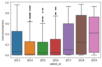
After that I’ve checked changes in features over time, only instrumentalness had some visible difference:
sns.boxplot(x=tracks_with_features_df.added_at.dt.year,
            y=tracks_with_features_df.instrumentalness)
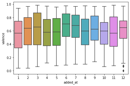
Then I had an idea to check seasonality and valence, and it kind of showed that in depressing months valence is a bit lower:
sns.boxplot(x=tracks_with_features_df.added_at.dt.month,
            y=tracks_with_features_df.valence)
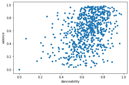
To play a bit more with data, I decided to check that danceability and valence might correlate:
tracks_with_features_df.plot(kind='scatter', x='danceability', y='valence')
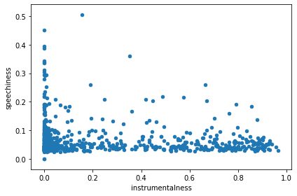
And to check that the data is meaningful, I checked instrumentalness vs speechiness, and those featues looked mutually exclusive as expected:
tracks_with_features_df.plot(kind='scatter', x='instrumentalness', y='speechiness')
Tracks difference and similarity
As I already had a bunch of features classifying tracks, it was hard not to make vectors out of them:
encode_fields = [
    'danceability',
    'energy',
    'key',
    'loudness',
    'mode',
    'speechiness',
    'acousticness',
    'instrumentalness',
    'liveness',
    'valence',
    'tempo',
    'duration_ms',
    'time_signature',
]

def encode(row):
    return np.array([
        (row[k] - tracks_with_features_df[k].min())
        / (tracks_with_features_df[k].max() - tracks_with_features_df[k].min())
        for k in encode_fields])

tracks_with_features_encoded_df = tracks_with_features_df.assign(
    encoded=tracks_with_features_df.apply(encode, axis=1))
Then I just calculated distance between every two tracks:
tracks_with_features_encoded_product_df = tracks_with_features_encoded_df \
    .assign(temp=0) \
    .merge(tracks_with_features_encoded_df.assign(temp=0), on='temp', how='left') \
    .drop(columns='temp')
tracks_with_features_encoded_product_df = tracks_with_features_encoded_product_df[
    tracks_with_features_encoded_product_df.id_x != tracks_with_features_encoded_product_df.id_y
]
tracks_with_features_encoded_product_df['merge_id'] = tracks_with_features_encoded_product_df \
    .apply(lambda row: ''.join(sorted([row['id_x'], row['id_y']])), axis=1)
tracks_with_features_encoded_product_df['distance'] = tracks_with_features_encoded_product_df \
    .apply(lambda row: np.linalg.norm(row['encoded_x'] - row['encoded_y']), axis=1)
After that I was able to get most similar songs/songs with the minimal distance, and it selected kind of similar songs:
tracks_with_features_encoded_product_df \
    .sort_values('distance') \
    .drop_duplicates('merge_id') \
    [['artist_x', 'name_x', 'release_date_x', 'artist_y', 'name_y', 'release_date_y', 'distance']] \
    .head(10)
| artist_x | name_x | release_date_x | artist_y | name_y | release_date_y | distance | |
|---|---|---|---|---|---|---|---|
| 84370 | Labyrinth Ear | Wild Flowers | 2010-11-21 | Labyrinth Ear | Navy Light | 2010-11-21 | 0.000000 |
| 446773 | YACHT | I Thought the Future Would Be Cooler | 2015-09-11 | ADULT. | Love Lies | 2013-05-13 | 0.111393 |
| 21963 | Ladytron | Seventeen | 2011-03-29 | The Juan Maclean | Give Me Every Little Thing | 2005-07-04 | 0.125358 |
| 11480 | Class Actress | Careful What You Say | 2010-02-09 | MGMT | Little Dark Age | 2017-10-17 | 0.128865 |
| 261780 | Queen of Japan | I Was Made For Loving You | 2001-10-02 | Midnight Juggernauts | Devil Within | 2007-10-02 | 0.131304 |
| 63257 | Pixies | Bagboy | 2013-09-09 | Kindness | That's Alright | 2012-03-16 | 0.146897 |
| 265792 | Datarock | Computer Camp Love | 2005-10-02 | Chromeo | Night By Night | 2010-09-21 | 0.147235 |
| 75359 | Midnight Juggernauts | Devil Within | 2007-10-02 | Lykke Li | I'm Good, I'm Gone | 2008-01-28 | 0.152680 |
| 105246 | ADULT. | Love Lies | 2013-05-13 | Dr. Alban | Sing Hallelujah! | 1992-05-04 | 0.154475 |
| 285180 | Gigamesh | Don't Stop | 2012-05-28 | Pet Shop Boys | Paninaro 95 - 2003 Remaster | 2003-10-02 | 0.156469 |
The most different songs weren’t that fun, as two songs were too different from the rest:
tracks_with_features_encoded_product_df \
    .sort_values('distance', ascending=False) \
    .drop_duplicates('merge_id') \
    [['artist_x', 'name_x', 'release_date_x', 'artist_y', 'name_y', 'release_date_y', 'distance']] \
    .head(10)
| artist_x | name_x | release_date_x | artist_y | name_y | release_date_y | distance | |
|---|---|---|---|---|---|---|---|
| 79324 | Labyrinth Ear | Navy Light | 2010-11-21 | Boy Harsher | Modulations | 2014-10-01 | 2.480206 |
| 84804 | Labyrinth Ear | Wild Flowers | 2010-11-21 | Boy Harsher | Modulations | 2014-10-01 | 2.480206 |
| 400840 | Charlotte Gainsbourg | Deadly Valentine - Soulwax Remix | 2017-11-10 | Labyrinth Ear | Navy Light | 2010-11-21 | 2.478183 |
| 84840 | Labyrinth Ear | Wild Flowers | 2010-11-21 | Charlotte Gainsbourg | Deadly Valentine - Soulwax Remix | 2017-11-10 | 2.478183 |
| 388510 | Ladytron | Paco! | 2001-10-02 | Labyrinth Ear | Navy Light | 2010-11-21 | 2.444927 |
| 388518 | Ladytron | Paco! | 2001-10-02 | Labyrinth Ear | Wild Flowers | 2010-11-21 | 2.444927 |
| 20665 | Factory Floor | Fall Back | 2013-01-15 | Labyrinth Ear | Navy Light | 2010-11-21 | 2.439136 |
| 20673 | Factory Floor | Fall Back | 2013-01-15 | Labyrinth Ear | Wild Flowers | 2010-11-21 | 2.439136 |
| 79448 | Labyrinth Ear | Navy Light | 2010-11-21 | La Femme | Runway | 2018-10-01 | 2.423574 |
| 84928 | Labyrinth Ear | Wild Flowers | 2010-11-21 | La Femme | Runway | 2018-10-01 | 2.423574 |
Then I calculated the most avarage songs, eg the songs with the least distance from every other song:
tracks_with_features_encoded_product_df \
    .groupby(['artist_x', 'name_x', 'release_date_x']) \
    .sum()['distance'] \
    .reset_index() \
    .sort_values('distance') \
    .head(10)
| artist_x | name_x | release_date_x | distance | |
|---|---|---|---|---|
| 48 | Beirut | No Dice | 2009-02-17 | 638.331257 |
| 591 | The Juan McLean | A Place Called Space | 2014-09-15 | 643.436523 |
| 347 | MGMT | Little Dark Age | 2017-10-17 | 645.959770 |
| 101 | Class Actress | Careful What You Say | 2010-02-09 | 646.488998 |
| 31 | Architecture In Helsinki | 2 Time | 2014-04-01 | 648.692344 |
| 588 | The Juan Maclean | Give Me Every Little Thing | 2005-07-04 | 648.878463 |
| 323 | Lindstrøm | Baby Can't Stop | 2009-10-26 | 652.212858 |
| 307 | Ladytron | Seventeen | 2011-03-29 | 652.759843 |
| 310 | Lauer | Mirrors (feat. Jasnau) | 2018-11-16 | 655.498535 |
| 451 | Pet Shop Boys | Always on My Mind | 1998-03-31 | 656.437048 |
And totally opposite thing – the most outstanding songs:
tracks_with_features_encoded_product_df \
    .groupby(['artist_x', 'name_x', 'release_date_x']) \
    .sum()['distance'] \
    .reset_index() \
    .sort_values('distance', ascending=False) \
    .head(10)
| artist_x | name_x | release_date_x | distance | |
|---|---|---|---|---|
| 665 | YACHT | Le Goudron - Long Version | 2012-05-25 | 2823.572387 |
| 300 | Labyrinth Ear | Navy Light | 2010-11-21 | 1329.234390 |
| 301 | Labyrinth Ear | Wild Flowers | 2010-11-21 | 1329.234390 |
| 57 | Blonde Redhead | For the Damaged Coda | 2000-06-06 | 1095.393120 |
| 616 | The Velvet Underground | After Hours | 1969-03-02 | 1080.491779 |
| 593 | The Knife | Forest Families | 2006-02-17 | 1040.114214 |
| 615 | The Space Lady | Major Tom | 2013-11-18 | 1016.881467 |
| 107 | CocoRosie | By Your Side | 2004-03-09 | 1015.970860 |
| 170 | El Perro Del Mar | Party | 2015-02-13 | 1012.163212 |
| 403 | Mr.Kitty | XIII | 2014-10-06 | 1010.115117 |
Conclusion
Although the dataset is a bit small, it was still fun to have a look at the data.
Gist with a jupyter notebook with even more boring stuff, can be reused by modifying credentials.