Recently, when I was having fun with algorithms exercises, I though, do I solve them correctly? So I thought that it would be neat to somehow find the complexity of an algorithm.
Gathering the data
The first idea was to use timeit and calculate complexity based on consumed time:
import timeit
from numpy.random import randint


def _get_data_set(size):
    return list(randint(1000, size=size))


def main(alist):
    for passnum in range(len(alist) - 1, 0, -1):
        for i in range(passnum):
            if alist[i] > alist[i + 1]:
                temp = alist[i]
                alist[i] = alist[i + 1]
                alist[i + 1] = temp


for size in range(1000, 10000, 1000):
    print(size, '=>', timeit.timeit('main(xs)',
                                    f'xs = _get_data_set({size})',
                                    globals=globals()))
1000 => 0.25852540601044893
2000 => 1.9087769229663536
3000 => 3.760379843064584
4000 => 5.552884255070239
5000 => 9.784064659965225
6000 => 10.014859249000438
7000 => 21.16908495896496
8000 => 19.5277360730106
9000 => 24.729382600053214
But it wasn’t much accurate and useful for small functions, required too big data set and required to run the function multiple times for acquiring meaningful data.
The second idea was to use cProfile:
from cProfile import Profile


profiler = Profile()
profiler.runcall(main, _get_data_set(1000))
profiler.print_stats()
         3 function calls in 0.269 seconds

   Ordered by: standard name

   ncalls  tottime  percall  cumtime  percall filename:lineno(function)
        1    0.269    0.269    0.269    0.269 t.py:43(main)
        1    0.000    0.000    0.000    0.000 {built-in method builtins.len}
        1    0.000    0.000    0.000    0.000 {method 'disable' of '_lsprof.Profiler' objects}
But it tracks only function calls and is useless for small algorithmic functions. So I found line_profiler line-by-line profiler:
from line_profiler import LineProfiler


profiler = LineProfiler(main)
profiler.runcall(main, _get_data_set(1000))
profiler.print_stats()
Total time: 2.21358 s
File: /home/nvbn/exp/complexity/t.py
Function: main at line 43

Line #      Hits         Time  Per Hit   % Time  Line Contents
==============================================================
    43                                           def main(alist):
    44      1000         1232      1.2      0.1      for passnum in range(len(alist) - 1, 0, -1):
    45    500499       557623      1.1     25.2          for i in range(passnum):
    46    499500       729304      1.5     32.9              if alist[i] > alist[i + 1]:
    47    243075       278005      1.1     12.6                  temp = alist[i]
    48    243075       334224      1.4     15.1                  alist[i] = alist[i + 1]
    49    243075       313194      1.3     14.1                  alist[i + 1] = temp
Which works fairly well for this task.
And as for guessing complexity we almost always need only the magnitude of growth, we can just calculate all hits, like:
def _get_hits(fn, *args, **kwargs):
    profiler = LineProfiler(fn)
    profiler.runcall(fn, *args, **kwargs)
    hits = 0
    for timing in profiler.get_stats().timings.values():
        for _, line_hits, _ in timing:
            hits += line_hits
    return hits


for size in range(100, 1000, 100):
    print(size, '=>', _get_hits(main, _get_data_set(size)))
100 => 17257
200 => 69872
300 => 159227
400 => 279847
500 => 429965
600 => 622175
700 => 852160
800 => 1130426
900 => 1418903
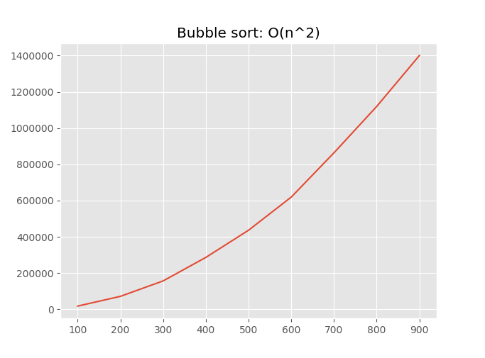
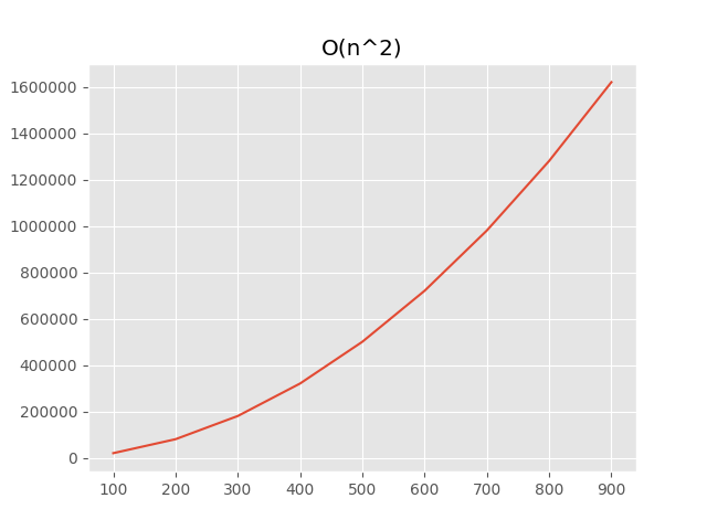
So to proof that it’s correct, we can visualize it with matplotlib:
import matplotlib.pyplot as plt


result = [(size, _get_hits(main, _get_data_set(size)))
          for size in range(100, 1000, 100)]

plt.style.use('ggplot')
plt.plot([size for size, _ in result],
         [hits for _, hits in result])
plt.title('Bubble sort: O(n^2)')
plt.show()
On the plot we can obviously see that the complexity is quadratic:
Finding complexity
For finding most the appropriate complexity, we need to have a special functions
like def get_score(hits: List[Tuple[int, int]]) -> int. And a complexity with the lowest score
will be the most appropriate.
Let’s start with constant complexity:
def constant(xs):
    result = 0
    for n in range(5):
        result += n
    return result


hits = [(size, _get_hits(constant, _get_data_set(size)))
        for size in range(100, 1000, 100)]
[(100, 13), (200, 13), (300, 13), (400, 13), (500, 13), (600, 13), (700, 13), (800, 13), (900, 13)]
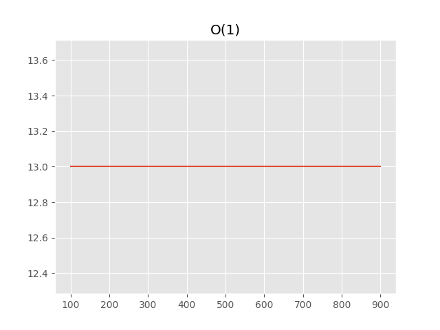
We can see, that hits count not depends at all on the size of the data set, so we can calculate the score by just summing diff with the first hit:
def get_constant_score(hits):
    return sum(abs(hits[0][1] - hit) for _, hit in hits[1:])


get_constant_score(hits)
0
The next is linear complexity:
def linear(xs):
    result = 0
    for x in xs:
        result += x
    return result


hits = [(size, _get_hits(linear, _get_data_set(size)))
        for size in range(100, 1000, 100)]
[(100, 203), (200, 403), (300, 603), (400, 803), (500, 1003), (600, 1203), (700, 1403), (800, 1603), (900, 1803)]
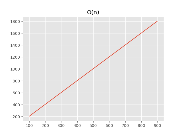
We can notice that the order of growth is linear, so we can use the similar approach as with constant complexity, but with growth instead of hits:
def _get_growth(hits):
    for hit_a, hit_b in zip(hits[:-1], hits[1:]):
        yield abs(hit_a - hit_b)


def get_linear_score(hits):
    hits = [hit for _, hit in hits]
    growth = list(_get_growth(hits))
    return sum(abs(growth[0] - grow) for grow in growth[1:])


get_linear_score(hits)
0
Now it’s time for quadratic complexity:
def quadratic(xs):
    result = 0
    for x in xs:
        for y in xs:
            result += x + y
    return result


hits = [(size, _get_hits(quadratic, _get_data_set(size)))
        for size in range(100, 1000, 100)]
[(100, 20203), (200, 80403), (300, 180603), (400, 320803), (500, 501003), (600, 721203), (700, 981403), (800, 1281603), (900, 1621803)]
It’s a bit more complicated in this case, the order of growth of the order of growth (like second derivative) should be the same:
def get_quadratic_score(hits):
    hits = [hit for _, hit in hits]
    growth = list(_get_growth(hits))
    growth_of_growth = list(_get_growth(growth))
    return sum(abs(growth_of_growth[0] - grow)
               for grow in growth_of_growth[1:])


get_quadratic_score(hits)
0
With similar approach detection of O(log(n)), O(n*log(n)) and etc can be implemented.
Usable public API
The code used above is only usable in REPL or a similar interactive environment. So let’s define simple and extensible API. First of all, complexity assumptions:
ComplexityLogEntry = NamedTuple('ComplexityLogEntry', [('size', int),
                                                       ('hits', int)])


class BaseComplexityAssumption(ABC):
    title = ''

    def __init__(self, log: List[ComplexityLogEntry]) -> None:
        self.log = log
        self.hits = [hit for _, hit in self.log]

    @abstractmethod
    def get_score(self) -> int:
        ...
So, for example, an assumption for constant complexity will be like:
class ConstantComplexityAssumption(BaseComplexityAssumption):
    title = 'O(1)'

    def get_score(self) -> int:
        return sum(abs(self.hits[0] - hit) for hit in self.hits[1:])
The next part of public API is Analyzer:
class Complexity:
    def __init__(self, title: str, log: List[ComplexityLogEntry]) -> None:
        ...

    def show_plot(self) -> 'Complexity':
        ...


T = TypeVar('T')


class BaseComplexityAnalyzer(Generic[T], ABC):
    title = ''

    @abstractmethod
    def get_data_set(self, size: int) -> T:
        ...

    @abstractmethod
    def run(self, data_set: T) -> None:
        ...

    @classmethod
    def calculate(cls, sizes: Iterable[int]) -> Complexity:
        ...

    ...
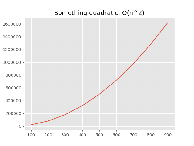
So we can analyze some quadratic algorithm very easily:
class SomethingQuadratic(BaseComplexityAnalyzer[int]):
    title = 'Something quadratic'

    def get_data_set(self, size) -> List[int]:
        from numpy.random import randint
        return list(randint(1000, size=size))

    def run(self, data_set: Iterable[int]) -> None:
        result = []
        for x in data_set:
            for y in data_set:
                result.append((x, y))


SomethingQuadratic \
    .calculate(range(100, 1000, 100)) \
    .show_plot()
And it works: