Welcome

Gene Kim, Kevin Behr, George Spafford: The Phoenix Project

Apr 24, 2019

book cover white Not so long ago I got recommended to read The Phoenix Project by Gene Kim, Kevin Behr and George Spafford, and I’ve got a bit of mixed feelings about the book.

The first part of the book is entertaining, as it shows that everything is bad and becoming even worse. It sounds like something from real life and reminds of some work situations.

The second part is still interesting, as it describes how they’re solving their problems in an iterative way, without going overboard.

The last part is kind of meh, too cheerful and happy, and like devops are going to solve all possible problems, and how magically everything works.

Sarah Guido, Andreas C. Müller: Introduction to Machine Learning with Python

Jan 31, 2019

book cover white Recently I’ve started to play in a data scientist a bit more and found that I’m not that much know machine learning basics, so I’ve decided to read Introduction to Machine Learning with Python by Sarah Guido and Andreas C. Müller. It’s a nice book, it explains fundamental concepts without going to deep and without requiring much of a math background. The book has a lot of simple synthetic and kind of real-life examples and covers a few popular use cases.

Although, in some chapters, it felt like reading a Jupyter notebook, but I’ve enjoyed an example with “this is how we get ants”.

Extracting popular topics from subreddits

Jan 07, 2019

Continuing playing with Reddit data, I thought that it might be fun to extract discussed topics from subreddits. My idea was: get comments from a subreddit, extract ngrams, calculate counts of ngrams, normalize counts, and subtract them from normalized counts of ngrams from a neutral set of comments.

Small-scale

For proving the idea on a smaller scale, I’ve fetched titles, texts and the first three levels of comments from top 1000 r/all posts (full code available in a gist), as it should have a lot of texts from different subreddits:

get_subreddit_df('all').head()

	id	subreddit	post_id	kind	text	created	score
0	7mjw12_title	all	7mjw12	title	My cab driver tonight was so excited to share ...	1.514459e+09	307861
1	7mjw12_selftext	all	7mjw12	selftext		1.514459e+09	307861
2	7mjw12_comment_druihai	all	7mjw12	comment	I want to make good humored inappropriate joke...	1.514460e+09	18336
3	7mjw12_comment_drulrp0	all	7mjw12	comment	Me too! It came out of nowhere- he was pretty ...	1.514464e+09	8853
4	7mjw12_comment_druluji	all	7mjw12	comment	Well, you got him to the top of Reddit, litera...	1.514464e+09	4749

Lemmatized texts, get all 1-3 words ngrams and counted them:

df = get_tokens_df(subreddit)  # Full code is in gist
df.head()

	token	amount
0	cab	84
1	driver	1165
2	tonight	360
3	excited	245
4	share	1793

Then I’ve normalized counts:

df['amount_norm'] = (df.amount - df.amount.mean()) / (df.amount.max() - df.amount.min())
df.head()

	token	amount	amount_norm
0	automate	493	0.043316
1	boring	108	0.009353
2	stuff	1158	0.101979
3	python	11177	0.985800
4	tinder	29	0.002384

And as the last step, I’ve calculated diff and got top 5 ngrams with texts from top 1000 posts from some random subreddits. Seems to be working for r/linux:

diff_tokens(tokens_dfs['linux'], tokens_dfs['all']).head()

	token	amount_diff	amount_norm_diff
5807	kde	3060.0	1.082134
2543	debian	1820.0	1.048817
48794	coc	1058.0	1.028343
9962	systemd	925.0	1.024769
11588	gentoo	878.0	1.023506

Also looks ok on r/personalfinance:

diff_tokens(tokens_dfs['personalfinance'], tokens_dfs['all']).head()

	token	amount_diff	amount_norm_diff
78063	vanguard	1513.0	1.017727
18396	etf	1035.0	1.012113
119206	checking account	732.0	1.008555
60873	direct deposit	690.0	1.008061
200917	joint account	679.0	1.007932

And kind of funny with r/drunk:

diff_tokens(tokens_dfs['drunk'], tokens_dfs['all']).head()

	token	amount_diff	amount_norm_diff
515158	honk honk honk	144.0	1.019149
41088	pbr	130.0	1.017247
49701	mo dog	129.0	1.017112
93763	cheap beer	74.0	1.009641
124756	birthday dude	61.0	1.007875

Seems to be working on this scale.

A bit larger scale

As the next iteration, I’ve decided to try the idea on three months of comments, which I was able to download as dumps from pushift.io.

Shaping the data

And it’s kind of a lot of data, even compressed:

$ du -sh raw_data/*
11G	raw_data/RC_2018-08.xz
10G	raw_data/RC_2018-09.xz
11G	raw_data/RC_2018-10.xz

Pandas basically doesn’t work on that scale, and unfortunately, I don’t have a personal Hadoop cluster. So I’ve reinvented a wheel a bit:

graph LR A[Reddit comments]-->B[Reddit comments wiht ngrams] B-->C[Ngrams partitioned by subreddit and day] C-->D[Counted partitioned ngrams]

The raw data is stored in line-delimited JSON, like:

$ xzcat raw_data/RC_2018-10.xz | head -n 2
{"archived":false,"author":"TistedLogic","author_created_utc":1312615878,"author_flair_background_color":null,"author_flair_css_class":null,"author_flair_richtext":[],"author_flair_template_id":null,"author_flair_text":null,"author_flair_text_color":null,"author_flair_type":"text","author_fullname":"t2_5mk6v","author_patreon_flair":false,"body":"Is it still r\/BoneAppleTea worthy if it's the opposite?","can_gild":true,"can_mod_post":false,"collapsed":false,"collapsed_reason":null,"controversiality":0,"created_utc":1538352000,"distinguished":null,"edited":false,"gilded":0,"gildings":{"gid_1":0,"gid_2":0,"gid_3":0},"id":"e6xucdd","is_submitter":false,"link_id":"t3_9ka1hp","no_follow":true,"parent_id":"t1_e6xu13x","permalink":"\/r\/Unexpected\/comments\/9ka1hp\/jesus_fking_woah\/e6xucdd\/","removal_reason":null,"retrieved_on":1539714091,"score":2,"send_replies":true,"stickied":false,"subreddit":"Unexpected","subreddit_id":"t5_2w67q","subreddit_name_prefixed":"r\/Unexpected","subreddit_type":"public"}
{"archived":false,"author":"misssaladfingers","author_created_utc":1536864574,"author_flair_background_color":null,"author_flair_css_class":null,"author_flair_richtext":[],"author_flair_template_id":null,"author_flair_text":null,"author_flair_text_color":null,"author_flair_type":"text","author_fullname":"t2_27d914lh","author_patreon_flair":false,"body":"I've tried and it's hit and miss. When it's good I feel more rested even though I've not slept well but sometimes it doesn't work","can_gild":true,"can_mod_post":false,"collapsed":false,"collapsed_reason":null,"controversiality":0,"created_utc":1538352000,"distinguished":null,"edited":false,"gilded":0,"gildings":{"gid_1":0,"gid_2":0,"gid_3":0},"id":"e6xucde","is_submitter":false,"link_id":"t3_9k8bp4","no_follow":true,"parent_id":"t1_e6xu9sk","permalink":"\/r\/insomnia\/comments\/9k8bp4\/melatonin\/e6xucde\/","removal_reason":null,"retrieved_on":1539714091,"score":1,"send_replies":true,"stickied":false,"subreddit":"insomnia","subreddit_id":"t5_2qh3g","subreddit_name_prefixed":"r\/insomnia","subreddit_type":"public"}

The first script add_ngrams.py reads lines of raw data from stdin, adds 1-3 lemmatized ngrams and writes lines in JSON to stdout. As the amount of data is huge, I’ve gzipped the output. It took around an hour to process month worth of comments on 12 CPU machine. Spawning more processes didn’t help as thw whole thing is quite CPU intense.

$ xzcat raw_data/RC_2018-10.xz | python3.7 add_ngrams.py | gzip > with_ngrams/2018-10.gz
$ zcat with_ngrams/2018-10.gz | head -n 2
{"archived": false, "author": "TistedLogic", "author_created_utc": 1312615878, "author_flair_background_color": null, "author_flair_css_class": null, "author_flair_richtext": [], "author_flair_template_id": null, "author_flair_text": null, "author_flair_text_color": null, "author_flair_type": "text", "author_fullname": "t2_5mk6v", "author_patreon_flair": false, "body": "Is it still r/BoneAppleTea worthy if it's the opposite?", "can_gild": true, "can_mod_post": false, "collapsed": false, "collapsed_reason": null, "controversiality": 0, "created_utc": 1538352000, "distinguished": null, "edited": false, "gilded": 0, "gildings": {"gid_1": 0, "gid_2": 0, "gid_3": 0}, "id": "e6xucdd", "is_submitter": false, "link_id": "t3_9ka1hp", "no_follow": true, "parent_id": "t1_e6xu13x", "permalink": "/r/Unexpected/comments/9ka1hp/jesus_fking_woah/e6xucdd/", "removal_reason": null, "retrieved_on": 1539714091, "score": 2, "send_replies": true, "stickied": false, "subreddit": "Unexpected", "subreddit_id": "t5_2w67q", "subreddit_name_prefixed": "r/Unexpected", "subreddit_type": "public", "ngrams": ["still", "r/boneappletea", "worthy", "'s", "opposite", "still r/boneappletea", "r/boneappletea worthy", "worthy 's", "'s opposite", "still r/boneappletea worthy", "r/boneappletea worthy 's", "worthy 's opposite"]}
{"archived": false, "author": "1-2-3RightMeow", "author_created_utc": 1515801270, "author_flair_background_color": null, "author_flair_css_class": null, "author_flair_richtext": [], "author_flair_template_id": null, "author_flair_text": null, "author_flair_text_color": null, "author_flair_type": "text", "author_fullname": "t2_rrwodxc", "author_patreon_flair": false, "body": "Nice! I\u2019m going out for dinner with him right and I\u2019ll check when I get home. I\u2019m very interested to read that", "can_gild": true, "can_mod_post": false, "collapsed": false, "collapsed_reason": null, "controversiality": 0, "created_utc": 1538352000, "distinguished": null, "edited": false, "gilded": 0, "gildings": {"gid_1": 0, "gid_2": 0, "gid_3": 0}, "id": "e6xucdp", "is_submitter": true, "link_id": "t3_9k9x6m", "no_follow": false, "parent_id": "t1_e6xsm3n", "permalink": "/r/Glitch_in_the_Matrix/comments/9k9x6m/my_boyfriend_and_i_lost_10_hours/e6xucdp/", "removal_reason": null, "retrieved_on": 1539714092, "score": 42, "send_replies": true, "stickied": false, "subreddit": "Glitch_in_the_Matrix", "subreddit_id": "t5_2tcwa", "subreddit_name_prefixed": "r/Glitch_in_the_Matrix", "subreddit_type": "public", "ngrams": ["nice", "go", "dinner", "right", "check", "get", "home", "interested", "read", "nice go", "go dinner", "dinner right", "right check", "check get", "get home", "home interested", "interested read", "nice go dinner", "go dinner right", "dinner right check", "right check get", "check get home", "get home interested", "home interested read"]}

The next script partition.py reads stdin and writes files like 2018-10-10_AskReddit with just ngrams to a folder passed as an argument.

$ zcat with_ngrams/2018-10.gz | python3.7 parition.py partitions
$ cat partitions/2018-10-10_AskReddit | head -n 5
"gt"
"money"
"go"
"administration"
"building"

For three months of comments it created a lot of files:

$ ls partitions | wc -l
2715472

After that I’ve counted ngrams in partitions with group_count.py:

$ python3.7 group_count.py partitions counted
$ cat counted/2018-10-10_AskReddit | head -n 5
["gt", 7010]
["money", 3648]
["go", 25812]
["administration", 108]
["building", 573]

As r/all isn’t a real subreddit and it’s not possible to get it from the dump, I’ve chosen r/AskReddit as a source of “neutral” ngrams, for that I’ve calculated the aggregated count of ngrams with aggreage_whole.py:

$ python3.7 aggreage_whole.py AskReddit > aggregated/askreddit_whole.json
$ cat aggregated/askreddit_whole.json | head -n 5
[["trick", 26691], ["people", 1638951], ["take", 844834], ["zammy", 10], ["wine", 17315], ["trick people", 515], ["people take", 10336], ["take zammy", 2], ["zammy wine", 2], ["trick people take", 4], ["people take zammy", 2]...

Playing with the data

First of all, I’ve read “neutral” ngrams, removed ngrams appeared less than 100 times as otherwise it wasn’t fitting in RAM and calculated normalized count:

whole_askreddit_df = pd.read_json('aggregated/askreddit_whole.json', orient='values')
whole_askreddit_df = whole_askreddit_df.rename(columns={0: 'ngram', 1: 'amount'})
whole_askreddit_df = whole_askreddit_df[whole_askreddit_df.amount > 99]
whole_askreddit_df['amount_norm'] = norm(whole_askreddit_df.amount)

	ngram	amount	amount_norm
0	trick	26691	0.008026
1	people	1638951	0.492943
2	take	844834	0.254098
4	wine	17315	0.005206
5	trick people	515	0.000153

To be sure that the idea is still valid, I’ve randomly checked r/television for 10th October:

television_10_10_df = pd \
    .read_json('counted/2018-10-10_television', lines=True) \
    .rename(columns={0: 'ngram', 1: 'amount'})
television_10_10_df['amount_norm'] = norm(television_10_10_df.amount)
television_10_10_df = television_10_10_df.merge(whole_askreddit_df, how='left', on='ngram', suffixes=('_left', '_right'))
television_10_10_df['diff'] = television_10_10_df.amount_norm_left - television_10_10_df.amount_norm_right
television_10_10_df \
    .sort_values('diff', ascending=False) \
    .head()

	ngram	amount_left	amount_norm_left	amount_right	amount_norm_right	diff
13	show	1299	0.699950	319715.0	0.096158	0.603792
32	season	963	0.518525	65229.0	0.019617	0.498908
19	character	514	0.276084	101931.0	0.030656	0.245428
4	episode	408	0.218849	81729.0	0.024580	0.194269
35	watch	534	0.286883	320204.0	0.096306	0.190578

And just for fun, limiting to trigrams:

television_10_10_df\
    [television_10_10_df.ngram.str.count(' ') >= 2] \
    .sort_values('diff', ascending=False) \
    .head()

	ngram	amount_left	amount_norm_left	amount_right	amount_norm_right	diff
11615	better call saul	15	0.006646	1033.0	0.000309	0.006337
36287	would make sense	11	0.004486	2098.0	0.000629	0.003857
7242	ca n't wait	12	0.005026	5396.0	0.001621	0.003405
86021	innocent proven guilty	9	0.003406	1106.0	0.000331	0.003075
151	watch first episode	8	0.002866	463.0	0.000137	0.002728

Seems to be ok, as the next step I’ve decided to get top 50 discussed topics for every available day:

r_television_by_day = diff_n_by_day(  # in the gist
    50, whole_askreddit_df, 'television', '2018-08-01', '2018-10-31',
    exclude=['r/television'],
)
r_television_by_day[r_television_by_day.date == "2018-10-05"].head()

	ngram	amount_left	amount_norm_left	amount_right	amount_norm_right	diff	date
3	show	906	0.725002	319715.0	0.096158	0.628844	2018-10-05
8	season	549	0.438485	65229.0	0.019617	0.418868	2018-10-05
249	character	334	0.265933	101931.0	0.030656	0.235277	2018-10-05
1635	episode	322	0.256302	81729.0	0.024580	0.231723	2018-10-05
418	watch	402	0.320508	320204.0	0.096306	0.224202	2018-10-05

Then I thought that it might be fun to get overall top topics from daily top topics and make a weekly heatmap with seaborn:

r_television_by_day_top_topics = r_television_by_day \
    .groupby('ngram') \
    .sum()['diff'] \
    .reset_index() \
    .sort_values('diff', ascending=False)

r_television_by_day_top_topics.head()

	ngram	diff
916	show	57.649622
887	season	37.241199
352	episode	22.752369
1077	watch	21.202295
207	character	15.599798

r_television_only_top_df = r_television_by_day \
    [['date', 'ngram', 'diff']] \
    [r_television_by_day.ngram.isin(r_television_by_day_top_topics.ngram.head(10))] \
    .groupby([pd.Grouper(key='date', freq='W-MON'), 'ngram']) \
    .mean() \
    .reset_index() \
    .sort_values('date')

pivot = r_television_only_top_df \
    .pivot(index='ngram', columns='date', values='diff') \
    .fillna(-1)

sns.heatmap(pivot, xticklabels=r_television_only_top_df.date.dt.week.unique())

r/television by week

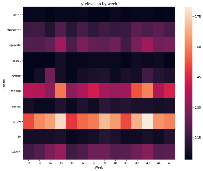
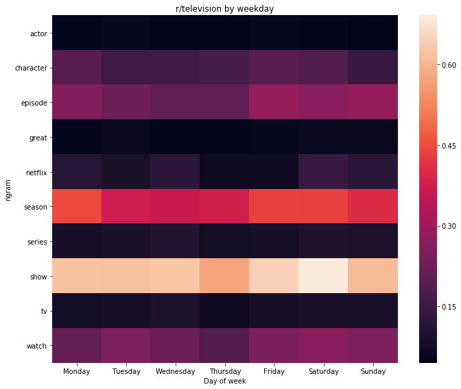
And it was quite boring, I’ve decided to try weekday heatmap, but it wasn’t better as topics were the same:

weekday_heatmap(r_television_by_day, 'r/television weekday')  # in the gist

r/television by weekday

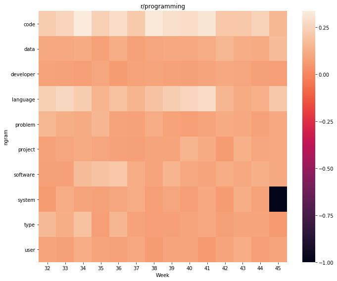
Heatmaps for r/programming are also boring:

r_programming_by_day = diff_n_by_day(  # in the gist
    50, whole_askreddit_df, 'programming', '2018-08-01', '2018-10-31',
    exclude=['gt', 'use', 'write'],  # selected manully
)
weekly_heatmap(r_programming_by_day, 'r/programming')

r/programming

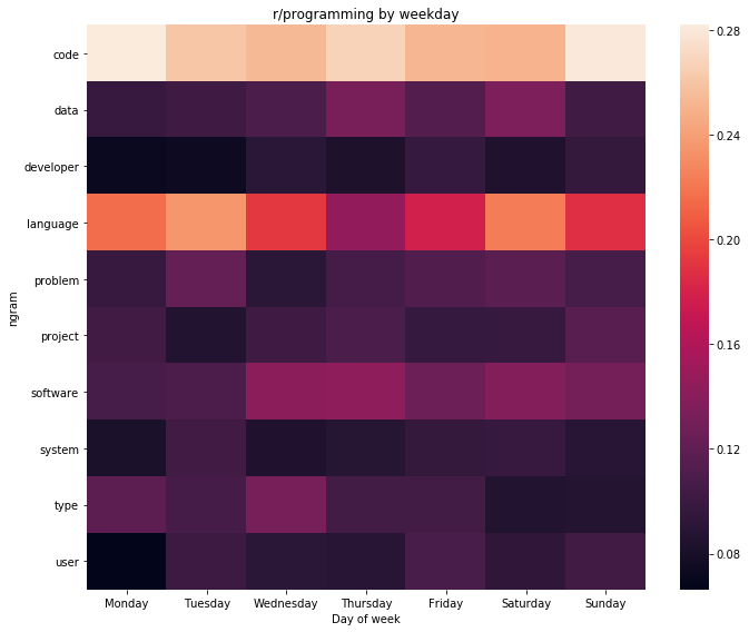
Although a heatmap by a weekday is a bit different:

weekday_heatmap(r_programming_by_day, 'r/programming by weekday')

r/programming by weekday

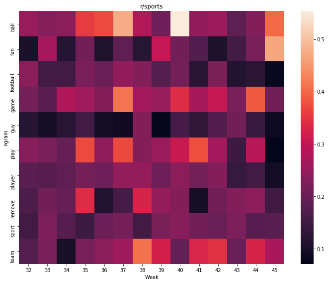
Another popular subreddit – r/sports:

r_sports_by_day = diff_n_by_day(
    50, whole_askreddit_df, 'sports', '2018-08-01', '2018-10-31',
    exclude=['r/sports'],
)
weekly_heatmap(r_sports_by_day, 'r/sports')

r/sports

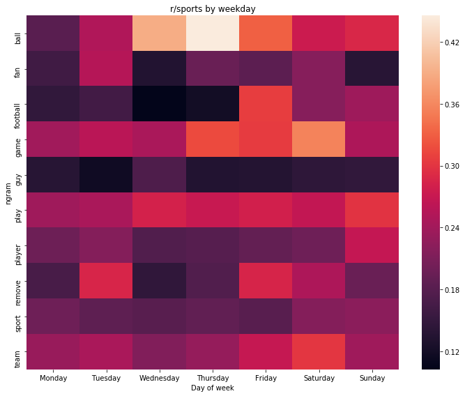
weekday_heatmap(r_sports_by_day, 'r/sports by weekday')

r/sports weekday

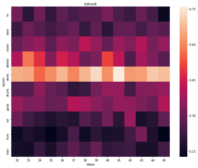
As the last subreddit for giggles – r/drunk:

r_drunk_by_day = diff_n_by_day(50, whole_askreddit_df, 'drunk', '2018-08-01', '2018-10-31')
weekly_heatmap(r_drunk_by_day, 'r/drunk')

r/drunk

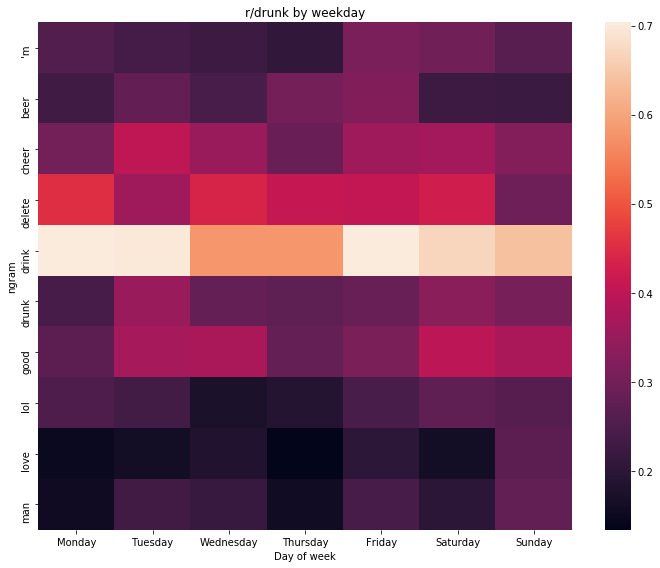
weekday_heatmap(r_drunk_by_day, "r/drunk by weekday")

r/drunk weekday

Conclusion

The idea kind of works for generic topics of subreddits, but can’t be used for finding trends.

Gist with everything.

Larry Gonick, Woollcott Smith: The Cartoon Guide to Statistics

Dec 11, 2018

book cover Recently I’ve noticed that I’m lacking some basics in statistics and got recommended to read The Cartoon Guide to Statistics by Larry Gonick and Woollcott Smith. The format of the book is a bit silly, but it covers a lot of topics and explains things in easy to understand way. The book has a lot of images and some kind of related stories for explained topics.

Although I’m not a big fan of the book format, the book seems to be nice.

Betsy Beyer, Niall Richard Murphy, David K. Rensin, Kent Kawahara and Stephen Thorne: The Site Reliability Workbook

Nov 29, 2018

book cover white More than two years ago I’ve read SRE Book, and now I finally found a time to read The Site Reliability Workbook by Betsy Beyer, Niall Richard Murphy, David K. Rensin, Kent Kawahara and Stephen Thorne. This book is more interesting, as it’s less idealistic and contains a lot of cases from real life. The book has examples of correct and wrong SLOs, explains how to properly implement alerts based on your error budget, and even a bit covers human part of SRE.

Overall SRE Workbook is one of the best books I’ve read recently, but it might be because the last few weeks I was doing related things at work.

Measuring community opinion: subreddits reactions to a link

Nov 28, 2018

As everyone knows a lot of subreddits are opinionated, so I thought that it might be interesting to measure the opinion of different subreddits. Not trying to start a holy war I’ve specifically decided to ignore r/worldnews and similar subreddits, and chose a semi-random topic – “Apu reportedly being written out of The Simpsons”.

For accessing Reddit API I’ve decided to use praw, because it already implements all OAuth related stuff and almost the same as REST API.

As a first step I’ve found all posts with that URL and populated pandas DataFrame:

[*posts] = reddit.subreddit('all').search(f"url:{url}", limit=1000)

posts_df = pd.DataFrame(
    [(post.id, post.subreddit.display_name, post.title, post.score,
      datetime.utcfromtimestamp(post.created_utc), post.url,
      post.num_comments, post.upvote_ratio)
     for post in posts],
    columns=['id', 'subreddit', 'title', 'score', 'created',
             'url', 'num_comments', 'upvote_ratio'])

posts_df.head()
       id         subreddit                                                                            title  score             created                                                                              url  num_comments  upvote_ratio
0  9rmz0o        television                                            Apu to be written out of The Simpsons   1455 2018-10-26 17:49:00  https://www.indiewire.com/2018/10/simpsons-drop-apu-character-adi-shankar-12...          1802          0.88
1  9rnu73        GamerGhazi                                 Apu reportedly being written out of The Simpsons     73 2018-10-26 19:30:39  https://www.indiewire.com/2018/10/simpsons-drop-apu-character-adi-shankar-12...            95          0.83
2  9roen1  worstepisodeever                                                     The Simpsons Writing Out Apu     14 2018-10-26 20:38:21  https://www.indiewire.com/2018/10/simpsons-drop-apu-character-adi-shankar-12...            22          0.94
3  9rq7ov          ABCDesis  ‘The Simpsons’ Is Eliminating Apu, But Producer Adi Shankar Found the Perfec...     26 2018-10-27 00:40:28  https://www.indiewire.com/2018/10/simpsons-drop-apu-character-adi-shankar-12...            11          0.84
4  9rnd6y         doughboys                                            Apu to be written out of The Simpsons     24 2018-10-26 18:34:58  https://www.indiewire.com/2018/10/simpsons-drop-apu-character-adi-shankar-12...             9          0.87

The easiest metric for opinion is upvote ratio:

posts_df[['subreddit', 'upvote_ratio']] \
    .groupby('subreddit') \
    .mean()['upvote_ratio'] \
    .reset_index() \
    .plot(kind='barh', x='subreddit', y='upvote_ratio',
          title='Upvote ratio', legend=False) \
    .xaxis \
    .set_major_formatter(FuncFormatter(lambda x, _: '{:.1f}%'.format(x * 100)))

But it doesn’t say us anything:

Upvote ratio

The most straightforward metric to measure is score:

posts_df[['subreddit', 'score']] \
    .groupby('subreddit') \
    .sum()['score'] \
    .reset_index() \
    .plot(kind='barh', x='subreddit', y='score', title='Score', legend=False)

Score by subreddit

A second obvious metric is a number of comments:

posts_df[['subreddit', 'num_comments']] \
    .groupby('subreddit') \
    .sum()['num_comments'] \
    .reset_index() \
    .plot(kind='barh', x='subreddit', y='num_comments',
          title='Number of comments', legend=False)

Number of comments

As absolute numbers can’t say us anything about an opinion of a subbreddit, I’ve decided to calculate normalized score and number of comments with data from the last 1000 of posts from the subreddit:

def normalize(post):
    [*subreddit_posts] = reddit.subreddit(post.subreddit.display_name).new(limit=1000)
    subreddit_posts_df = pd.DataFrame([(post.id, post.score, post.num_comments)
                                       for post in subreddit_posts],
                                      columns=('id', 'score', 'num_comments'))

    norm_score = ((post.score - subreddit_posts_df.score.mean())
                  / (subreddit_posts_df.score.max() - subreddit_posts_df.score.min()))
    norm_num_comments = ((post.num_comments - subreddit_posts_df.num_comments.mean())
                         / (subreddit_posts_df.num_comments.max() - subreddit_posts_df.num_comments.min()))

    return norm_score, norm_num_comments

normalized_vals = pd \
    .DataFrame([normalize(post) for post in posts],
               columns=['norm_score', 'norm_num_comments']) \
    .fillna(0)

posts_df[['norm_score', 'norm_num_comments']] = normalized_vals

And look at the popularity of the link based on the numbers:

posts_df[['subreddit', 'norm_score', 'norm_num_comments']] \
    .groupby('subreddit') \
    .sum()[['norm_score', 'norm_num_comments']] \
    .reset_index() \
    .rename(columns={'norm_score': 'Normalized score',
                     'norm_num_comments': 'Normalized number of comments'}) \
    .plot(kind='barh', x='subreddit',title='Normalized popularity')

Normalized popularity

As in different subreddits a link can be shared with a different title with totally different sentiments, it seemed interesting to do sentiment analysis on titles:

sid = SentimentIntensityAnalyzer()

posts_sentiments = posts_df.title.apply(sid.polarity_scores).apply(pd.Series)
posts_df = posts_df.assign(title_neg=posts_sentiments.neg,
                           title_neu=posts_sentiments.neu,
                           title_pos=posts_sentiments.pos,
                           title_compound=posts_sentiments['compound'])

And notice that people are using the same title almost every time:

posts_df[['subreddit', 'title_neg', 'title_neu', 'title_pos', 'title_compound']] \
    .groupby('subreddit') \
    .sum()[['title_neg', 'title_neu', 'title_pos', 'title_compound']] \
    .reset_index() \
    .rename(columns={'title_neg': 'Title negativity',
                     'title_pos': 'Title positivity',
                     'title_neu': 'Title neutrality',
                     'title_compound': 'Title sentiment'}) \
    .plot(kind='barh', x='subreddit', title='Title sentiments', legend=True)

Title sentiments

Sentiments of a title isn’t that interesting, but it might be much more interesting for comments. I’ve decided to only handle root comments as replies to comments might be totally not related to post subject, and they’re making everything more complicated. For comments analysis I’ve bucketed them to five buckets by compound value, and calculated mean normalized score and percentage:

posts_comments_df = pd \
    .concat([handle_post_comments(post) for post in posts]) \  # handle_post_comments is huge and available in the gist
    .fillna(0)

>>> posts_comments_df.head()
      key  root_comments_key  root_comments_neg_neg_amount  root_comments_neg_neg_norm_score  root_comments_neg_neg_percent  root_comments_neg_neu_amount  root_comments_neg_neu_norm_score  root_comments_neg_neu_percent  root_comments_neu_neu_amount  root_comments_neu_neu_norm_score  root_comments_neu_neu_percent  root_comments_pos_neu_amount  root_comments_pos_neu_norm_score  root_comments_pos_neu_percent  root_comments_pos_pos_amount  root_comments_pos_pos_norm_score  root_comments_pos_pos_percent root_comments_post_id
0  9rmz0o                  0                          87.0                         -0.005139                       0.175758                          98.0                          0.019201                       0.197980                         141.0                         -0.007125                       0.284848                          90.0                         -0.010092                       0.181818                            79                          0.006054                       0.159596                9rmz0o
0  9rnu73                  0                          12.0                          0.048172                       0.134831                          15.0                         -0.061331                       0.168539                          35.0                         -0.010538                       0.393258                          13.0                         -0.015762                       0.146067                            14                          0.065402                       0.157303                9rnu73
0  9roen1                  0                           9.0                         -0.094921                       0.450000                           1.0                          0.025714                       0.050000                           5.0                          0.048571                       0.250000                           0.0                          0.000000                       0.000000                             5                          0.117143                       0.250000                9roen1
0  9rq7ov                  0                           1.0                          0.476471                       0.100000                           2.0                         -0.523529                       0.200000                           0.0                          0.000000                       0.000000                           1.0                         -0.229412                       0.100000                             6                          0.133333                       0.600000                9rq7ov
0  9rnd6y                  0                           0.0                          0.000000                       0.000000                           0.0                          0.000000                       0.000000                           0.0                          0.000000                       0.000000                           5.0                         -0.027778                       0.555556                             4                          0.034722                       0.444444                9rnd6y

So now we can get a percent of comments by sentiments buckets:

percent_columns = ['root_comments_neg_neg_percent',
                   'root_comments_neg_neu_percent', 'root_comments_neu_neu_percent',
                   'root_comments_pos_neu_percent', 'root_comments_pos_pos_percent']

posts_with_comments_df[['subreddit'] + percent_columns] \
    .groupby('subreddit') \
    .mean()[percent_columns] \
    .reset_index() \
    .rename(columns={column: column[13:-7].replace('_', ' ')
                     for column in percent_columns}) \
    .plot(kind='bar', x='subreddit', legend=True,
          title='Percent of comments by sentiments buckets') \
    .yaxis \
    .set_major_formatter(FuncFormatter(lambda y, _: '{:.1f}%'.format(y * 100)))

It’s easy to spot that on less popular subreddits comments are more opinionated:

Comments sentiments

The same can be spotted with mean normalized scores:

norm_score_columns = ['root_comments_neg_neg_norm_score',
                      'root_comments_neg_neu_norm_score',
                      'root_comments_neu_neu_norm_score',
                      'root_comments_pos_neu_norm_score',
                      'root_comments_pos_pos_norm_score']

posts_with_comments_df[['subreddit'] + norm_score_columns] \
    .groupby('subreddit') \
    .mean()[norm_score_columns] \
    .reset_index() \
    .rename(columns={column: column[13:-10].replace('_', ' ')
                     for column in norm_score_columns}) \
    .plot(kind='bar', x='subreddit', legend=True,
          title='Mean normalized score of comments by sentiments buckets')

Comments normalized score

Although those plots are fun even with that link, it’s more fun with something more controversial. I’ve picked one of the recent posts from r/worldnews, and it’s easy to notice that different subreddits present the news in a different way:

Hot title sentiment

And comments are rated differently, some subreddits are more neutral, some definitely not:

Hot title sentiment

Gist with full source code.

Analysing the trip to South America with a bit of image recognition

Nov 21, 2018

Back in September, I had a three weeks trip to South America. While planning the trip I was using sort of data mining to select the most optimal flights and it worked well. To continue following the data-driven approach (more buzzwords), I’ve decided to analyze the data I’ve collected during the trip.

Unfortunately, I was traveling without local sim-card and almost without internet, I can’t use Google Location History as in the fun research about the commute. But at least I have tweets and a lot of photos.

At first, I’ve reused old code (more internal linking) and extracted information about flights from tweets:

all_tweets = pd.DataFrame(
    [(tweet.text, tweet.created_at) for tweet in get_tweets()],  # get_tweets available in the gist
    columns=['text', 'created_at'])

tweets_in_dates = all_tweets[
    (all_tweets.created_at > datetime(2018, 9, 8)) & (all_tweets.created_at < datetime(2018, 9, 30))]

flights_tweets = tweets_in_dates[tweets_in_dates.text.str.upper() == tweets_in_dates.text]

flights = flights_tweets.assign(start=lambda df: df.text.str.split('✈').str[0],
                                finish=lambda df: df.text.str.split('✈').str[-1]) \
                        .sort_values('created_at')[['start', 'finish', 'created_at']]

>>> flights
   start finish          created_at
AMS   ️ LIS 2018-09-08 05:00:32
LIS   ️ GIG 2018-09-08 11:34:14
SDU   ️ EZE 2018-09-12 23:29:52
EZE   ️ SCL 2018-09-16 17:30:01
SCL   ️ LIM 2018-09-19 16:54:13
LIM   ️ MEX 2018-09-22 20:43:42
MEX   ️ CUN 2018-09-25 19:29:04
CUN   ️ MAN 2018-09-29 20:16:11

Then I’ve found a json dump with airports, made a little hack with replacing Ezeiza with Buenos-Aires and found cities with lengths of stay from flights:

flights = flights.assign(
    start=flights.start.apply(lambda code: iata_to_city[re.sub(r'\W+', '', code)]),  # Removes leftovers of emojis, iata_to_city available in the gist
    finish=flights.finish.apply(lambda code: iata_to_city[re.sub(r'\W+', '', code)]))
cities = flights.assign(
    spent=flights.created_at - flights.created_at.shift(1),
    city=flights.start,
    arrived=flights.created_at.shift(1),
)[["city", "spent", "arrived"]]
cities = cities.assign(left=cities.arrived + cities.spent)[cities.spent.dt.days > 0]

>>> cities
              city           spent             arrived                left
17  Rio De Janeiro 4 days 11:55:38 2018-09-08 11:34:14 2018-09-12 23:29:52
16  Buenos-Aires   3 days 18:00:09 2018-09-12 23:29:52 2018-09-16 17:30:01
15  Santiago       2 days 23:24:12 2018-09-16 17:30:01 2018-09-19 16:54:13
14  Lima           3 days 03:49:29 2018-09-19 16:54:13 2018-09-22 20:43:42
13  Mexico City    2 days 22:45:22 2018-09-22 20:43:42 2018-09-25 19:29:04
11  Cancun         4 days 00:47:07 2018-09-25 19:29:04 2018-09-29 20:16:11

>>> cities.plot(x="city", y="spent", kind="bar",
                legend=False, title='Cities') \
          .yaxis.set_major_formatter(formatter)  # Ugly hack for timedelta formatting, more in the gist

Cities

Now it’s time to work with photos. I’ve downloaded all photos from Google Photos, parsed creation dates from Exif, and “joined” them with cities by creation date:

raw_photos = pd.DataFrame(list(read_photos()), columns=['name', 'created_at'])  # read_photos available in the gist

photos_cities = raw_photos.assign(key=0).merge(cities.assign(key=0), how='outer')
photos = photos_cities[
    (photos_cities.created_at >= photos_cities.arrived)
    & (photos_cities.created_at <= photos_cities.left)
]

>>> photos.head()
                          name          created_at  key            city           spent             arrived                left
 photos/20180913_183207.jpg 2018-09-13 18:32:07  0    Buenos-Aires   3 days 18:00:09 2018-09-12 23:29:52 2018-09-16 17:30:01
 photos/20180909_141137.jpg 2018-09-09 14:11:36  0    Rio De Janeiro 4 days 11:55:38 2018-09-08 11:34:14 2018-09-12 23:29:52
photos/20180917_162240.jpg 2018-09-17 16:22:40  0    Santiago       2 days 23:24:12 2018-09-16 17:30:01 2018-09-19 16:54:13
photos/20180923_161707.jpg 2018-09-23 16:17:07  0    Mexico City    2 days 22:45:22 2018-09-22 20:43:42 2018-09-25 19:29:04
photos/20180917_111251.jpg 2018-09-17 11:12:51  0    Santiago       2 days 23:24:12 2018-09-16 17:30:01 2018-09-19 16:54:13

After that I’ve got the amount of photos by city:

photos_by_city = photos \
    .groupby(by='city') \
    .agg({'name': 'count'}) \
    .rename(columns={'name': 'photos'}) \
    .reset_index()

>>> photos_by_city
             city  photos
0  Buenos-Aires    193
1  Cancun          292
2  Lima            295
3  Mexico City     256
4  Rio De Janeiro  422
5  Santiago        267
>>> photos_by_city.plot(x='city', y='photos', kind="bar",
                        title='Photos by city', legend=False)

Cities

Let’s go a bit deeper and use image recognition, to not reinvent the wheel I’ve used a slightly modified version of TensorFlow imagenet tutorial example and for each photo find what’s on it:

classify_image.init()
tags = tagged_photos.name\
    .apply(lambda name: classify_image.run_inference_on_image(name, 1)[0]) \
    .apply(pd.Series)

tagged_photos = photos.copy()
tagged_photos[['tag', 'score']] = tags.apply(pd.Series)
tagged_photos['tag'] = tagged_photos.tag.apply(lambda tag: tag.split(', ')[0])

>>> tagged_photos.head()
                          name          created_at  key            city           spent             arrived                left       tag     score
 photos/20180913_183207.jpg 2018-09-13 18:32:07  0    Buenos-Aires   3 days 18:00:09 2018-09-12 23:29:52 2018-09-16 17:30:01  cinema    0.164415
 photos/20180909_141137.jpg 2018-09-09 14:11:36  0    Rio De Janeiro 4 days 11:55:38 2018-09-08 11:34:14 2018-09-12 23:29:52  pedestal  0.667128
photos/20180917_162240.jpg 2018-09-17 16:22:40  0    Santiago       2 days 23:24:12 2018-09-16 17:30:01 2018-09-19 16:54:13  cinema    0.225404
photos/20180923_161707.jpg 2018-09-23 16:17:07  0    Mexico City    2 days 22:45:22 2018-09-22 20:43:42 2018-09-25 19:29:04  obelisk   0.775244
photos/20180917_111251.jpg 2018-09-17 11:12:51  0    Santiago       2 days 23:24:12 2018-09-16 17:30:01 2018-09-19 16:54:13  seashore  0.24720

So now it’s possible to find things that I’ve taken photos of the most:

photos_by_tag = tagged_photos \
    .groupby(by='tag') \
    .agg({'name': 'count'}) \
    .rename(columns={'name': 'photos'}) \
    .reset_index() \
    .sort_values('photos', ascending=False) \
    .head(10)

>>> photos_by_tag
            tag  photos
seashore    276   
 monastery   142   
 lakeside    116   
 palace      115   
  alp         86    
 obelisk     72    
promontory  50    
sandbar     49    
 bell cote   43    
 cliff       42
>>> photos_by_tag.plot(x='tag', y='photos', kind='bar',
                       legend=False, title='Popular tags')

Popular tags

Then I was able to find what I was taking photos of by city:

popular_tags = photos_by_tag.head(5).tag
popular_tagged = tagged_photos[tagged_photos.tag.isin(popular_tags)]
not_popular_tagged = tagged_photos[~tagged_photos.tag.isin(popular_tags)].assign(
    tag='other')
by_tag_city = popular_tagged \
    .append(not_popular_tagged) \
    .groupby(by=['city', 'tag']) \
    .count()['name'] \
    .unstack(fill_value=0)

>>> by_tag_city
tag             alp  lakeside  monastery  other  palace  seashore
city                                                             
Buenos-Aires    5    1         24         123    30      10      
Cancun          0    19        6          153    4       110     
Lima            0    25        42         136    38      54      
Mexico City     7    9         26         197    5       12      
Rio De Janeiro  73   45        17         212    4       71      
Santiago        1    17        27         169    34      19     
>>> by_tag_city.plot(kind='bar', stacked=True)

Tags by city

Although the most common thing on this plot is “other”, it’s still fun.

Gist with full sources.

Holden Karau, Rachel Warren: High Performance Spark

Oct 15, 2018

book cover white Recently I’ve started to use Spark more and more, so I’ve decided to read something about it. High Performance Spark by Holden Karau and Rachel Warren looked like an interesting book, and I already had it from some HIB bundle. The book is quite short, but it covers a lot of topics. It has a lot of technics to make Spark faster and avoid common bottlenecks with explanation and sometimes even going down to Spark internals. Although I’m mostly using PySpark and almost everything in the book is in Scala, it was still useful as API is mostly the same.

Some parts of High Performance Spark are like config key/param – sort of documentation, but most of the book is ok.

Video from subtitles or Bob's Burgers to The Simpsons with TensorFlow

Aug 30, 2018

Bob's Burgers to The Simpsons

Back in June I’ve played a bit with subtitles and tried to generate a filmstrip, it wasn’t that much successful, but it was fun. So I decided to try to go deeper and generate a video from subtitles. The main idea is to get phrases from a part of some video, get the most similar phrases from another video and generate something.

As the “enemy” I’ve decided to use a part from Bob’s Burgers Tina-rannosaurus Wrecks episode:

As the source, I’ve decided to use The Simpsons, as they have a lot of episodes and Simpsons Already Did It whatever. I somehow have 671 episode and managed to get perfectly matching subtitles for 452 of them.

TLDR: It was fun, but the result is meh at best:

Initially, I was planning to use Friends and Seinfeld but the result was even worse.

As the first step I’ve parsed subtitles (boring, available in the gist) and created a mapping from phrases and “captions” (subtitles parts with timing and additional data) and a list of phrases from all available subtitles:

data_text2captions = defaultdict(lambda: [])
for season in root.glob('*'):
    if season.is_dir():
        for subtitles in season.glob('*.srt'):
            for caption in read_subtitles(subtitles.as_posix()):
                data_text2captions[caption.text].append(caption)

data_texts = [*data_text2captions]

>>> data_text2captions["That's just a dog in a spacesuit!"]
[Caption(path='The Simpsons S13E06 She of Little Faith.srt', start=127795000, length=2544000, text="That's just a dog in a spacesuit!")]
>>> data_texts[0]
'Give up, Mr. Simpson! We know you have the Olympic torch!'

After that I’ve found subtitles for the Bob’s Burgers episode and manually selected parts from the part of the episode that I’ve used as the “enemy” and processed them in a similar way:

play = [*read_subtitles('Bobs.Burgers.S03E07.HDTV.XviD-AFG.srt')][1:54]
play_text2captions = defaultdict(lambda: [])
for caption in play:
    play_text2captions[caption.text].append(caption)

play_texts = [*play_text2captions]

>>> play_text2captions[ 'Who raised you?']
[Caption(path='Bobs.Burgers.S03E07.HDTV.XviD-AFG.srt', start=118605000, length=1202000, text='Who raised you?')]
>>> play_texts[0]
"Wow, still can't believe this sale."

Then I’ve generated vectors for all phrases with TensorFlow’s The Universal Sentence Encoder and used cosine similarity to get most similar phrases:

module_url = "https://tfhub.dev/google/universal-sentence-encoder/2"
embed = hub.Module(module_url)

vec_a = tf.placeholder(tf.float32, shape=None)
vec_b = tf.placeholder(tf.float32, shape=None)

normalized_a = tf.nn.l2_normalize(vec_a, axis=1)
normalized_b = tf.nn.l2_normalize(vec_b, axis=1)
sim_scores = -tf.acos(tf.reduce_sum(tf.multiply(normalized_a, normalized_b), axis=1))


def get_similarity_score(text_vec_a, text_vec_b):
    emba, embb, scores = session.run(
        [normalized_a, normalized_b, sim_scores],
        feed_dict={
            vec_a: text_vec_a,
            vec_b: text_vec_b
        })
    return scores


def get_most_similar_text(vec_a, data_vectors):
    scores = get_similarity_score([vec_a] * len(data_texts), data_vectors)
    return data_texts[sorted(enumerate(scores), key=lambda score: -score[1])[3][0]]


with tf.Session() as session:
    session.run([tf.global_variables_initializer(), tf.tables_initializer()])
    data_vecs, play_vecs = session.run([embed(data_texts), embed(play_texts)])
    data_vecs = np.array(data_vecs).tolist()
    play_vecs = np.array(play_vecs).tolist()

    similar_texts = {play_text: get_most_similar_text(play_vecs[n], data_vecs)
                     for n, play_text in enumerate(play_texts)}

>> similar_texts['Is that legal?']
"- [Gasping] - Uh, isn't that illegal?"
>>> similar_texts['(chuckling): Okay, okay.']
'[ Laughing Continues ] All right. Okay.

Looks kind of relevant, right? Unfortunately only phrase by phrase.

After that, I’ve cut parts of The Simpsons episodes for matching phrases. This part was a bit complicated, because without a force re-encoding (with the same encoding) and setting a framerate (with kind of the same framerate with most of the videos) it was producing unplayable videos:

def generate_parts():
    for n, caption in enumerate(play):
        similar = similar_texts[caption.text]
        similar_caption = sorted(
            data_text2captions[similar],
            key=lambda maybe_similar: abs(caption.length - maybe_similar.length),
            reverse=True)[0]

        yield Part(
            video=similar_caption.path.replace('.srt', '.mp4'),
            start=str(timedelta(microseconds=similar_caption.start))[:-3],
            end=str(timedelta(microseconds=similar_caption.length))[:-3],
            output=Path(output_dir).joinpath(f'part_{n}.mp4').as_posix())


parts = [*generate_parts()]
for part in parts:
    call(['ffmpeg', '-y', '-i', part.video,
          '-ss', part.start, '-t', part.end,
          '-c:v', 'libx264', '-c:a', 'aac', '-strict', 'experimental',
          '-vf', 'fps=30',
          '-b:a', '128k', part.output])

>>> parts[0]
Part(video='The Simpsons S09E22 Trash of the Titans.mp4', start='0:00:31.531', end='0:00:03.003', output='part_0.mp4')

And at the end I’ve generated a special file for the FFmpeg concat and concatenated the generated parts (also with re-encoding):

concat = '\n'.join(f"file '{part.output}'" for part in parts) + '\n'
with open('concat.txt', 'w') as f:
    f.write(concat)

➜ cat concat.txt | head -n 5
file 'parts/part_0.mp4'
file 'parts/part_1.mp4'
file 'parts/part_2.mp4'
file 'parts/part_3.mp4'
file 'parts/part_4.mp4'

call(['ffmpeg', '-y', '-safe', '0', '-f', 'concat', '-i', 'concat.txt',
      '-c:v', 'libx264', '-c:a', 'aac', '-strict', 'experimental',
      '-vf', 'fps=30', 'output.mp4'])

As the result is kind of meh, but it was fun, I’m going to try to do that again with a bigger dataset, even working with FFmpeg wasn’t fun at all.

Gist with full sources.

Christina Wodtke: Introduction to OKRs

Aug 16, 2018

book cover For a better understanding of OKRs, I’ve decided to read Introduction to OKRs by Christina Wodtke. It’s a very short book, but it explains why and how to set OKRs, and how to keep track of them. The book isn’t deep or something, but it contains almost everything I wanted to know about OKRs.

In contrast with some longer books, it’s very nice to read something that’s not trying to repeat the same content ten times all over the book.

« Older Posts Newer Posts »