Sam Newman: Monolith To Microservices


book cover white Recently I decided to up my “microservices” game a bit and read Monolith To Microservices by Sam Newman. I enjoyed this book more than the first microservices book, it’s not so upbeat and cheerful, and doesn’t have this annoying “everything should be on microservices” vibe, it even sometimes suggests that something might be better not as a microservice. Apart from that, the book covers a bunch of patterns for gradual extraction of parts of a monolith to a few microservices in an iteretive way. It also covers a few ways to separate the storage without breaking existing applications.
Overall for me it was interesting reading.

Alex Petrov: Database Internals


book cover white A few months ago I was a bit hyped about Database Internals by Alex Petrov and recently I had time to finally read it. And it’s a nice book. The first part of the book has lots of trees and covers the storage side of databases both persistent and in-memory with examples from actual databases but without going too deep in specific database implementation details. The second part is about distributed systems and shows what and why is used in different databases. It’s also a bit more generic as it can be applied not only to databases.

At least for me, it was a good reading on system design and architecture.

Tyler Akidau, Slava Chernyak, Reuven Lax: Streaming Systems


book cover white Recently I started to go a bit deeper in data processing and decided that it would be nice to read Streaming Systems by Tyler Akidau, Slava Chernyak, and Reuven Lax. It covers fundamentals and inside machinery of streaming systems, with explanations and examples. The book also has a bunch of nice gifs that help to understand how everything works. I also enjoyed the last chapter with a brief history of big data processing and some sort of explanation of why all those things created the way they created.
From the not so nice part sometimes the book feels a bit too much Google tech stack centric, and the images in the book are sometimes hard to understand, but gifs on the book’s website solved that for me.

Sound lights with Spotify and ESP8266


As unfortunately my old fancy sound lights setup only works on Linux, it stopped working after I switched to a new laptop. So I decided to make a cross-platform solution.

TLDR: Source code of the desktop app, ESP8266 “firmware”, a jupyter notebook with a preresearch and a video of sound lights in action (the best my phone can do):


Lights colors from audio

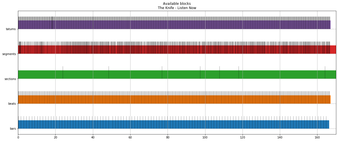
Apparently, it’s not so easy to capture and analyze audio stream from a random music app on macOS, so I chose a bit of vendor locked solution with a precalculated track analysis from Spotify API. The API provides a bunch of differently sized intervals with characteristics like loudness, mode and etc:

Available blocks

By trial and error and some random changes, I came up with a function that returns a list of tuples representing RGB colors. It’s not something fancy or at least correct, but can produce different colors and works fast enough:

def get_current_colors(t):
    segment = get_current_segmnet(t)
    section = get_current_section(t)
    beat = get_current_beat(t)

    beat_color = BASE_COLOR_MULTIPLIER * (t - beat['start'] + beat['duration']) / beat['duration']
    tempo_color = BASE_COLOR_MULTIPLIER * scale_tempo(section['tempo'])
    pitch_colors = [BASE_COLOR_MULTIPLIER * p for p in segment['pitches']]

    loudness_multiplier = 1 + LOUDNESS_MULTIPLIER * scale_loudness(section['loudness'])

    colors = ((beat_color * loudness_multiplier,
                tempo_color * loudness_multiplier,
                pitch_colors[n // (leds // 12)] * loudness_multiplier)
                for n in range(leds))

    if section['mode'] == 0:
        order = (0, 1, 2)
    elif section['mode'] == 1:
        order = (1, 2, 0)
    else:
        order = (2, 0, 1)

    ordered_colors = ((color[order[0]], color[order[1]], color[order[2]])
                        for color in colors)

    return [_scale_pixel(color) for color in ordered_colors]

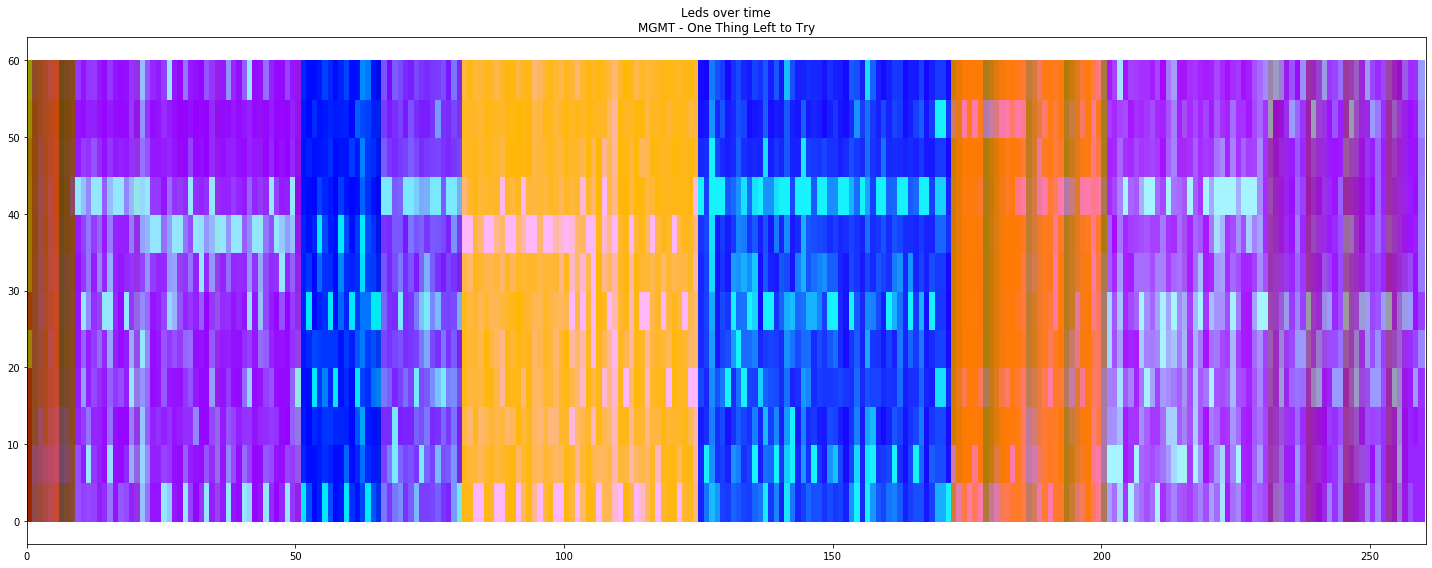
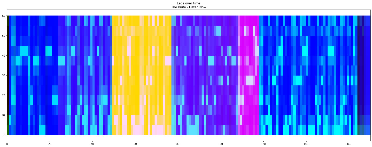
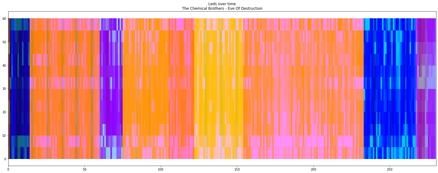
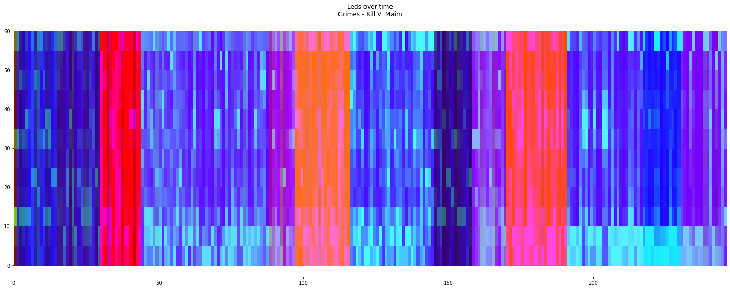
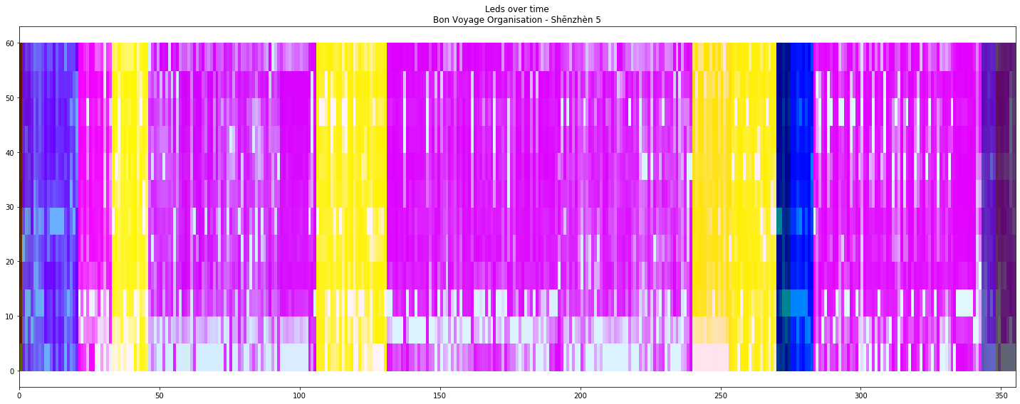
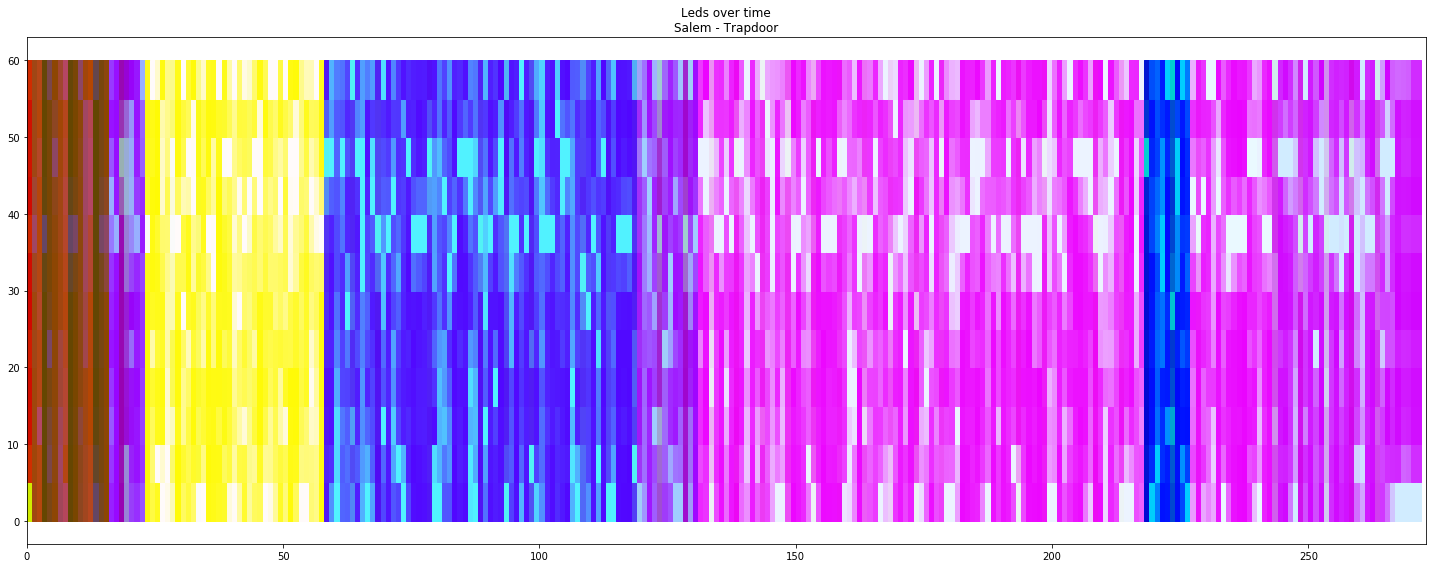
To ensure that it works I ran it on a bunch of songs with a 60 “LEDs” column for an each second:

MGMT - One Thing Left to Try The Knife - Listen Now The Chemical Brothers - Eve Of Destruction Grimes - Kill V. Maim Bon Voyage Organisation - Shenzhen V Salem - Trapdoor

It looks different enough and not that ugly for different songs and different parts of songs.

The full jupyter notebook available in the gist.

Led strip and EPS8266

The EPS8266 part is really easy, it listens UDP on 42424, waits for 180 bytes and changes colors of 60 LEDs strip with NeoPixels MicroPython library:

np = neopixel.NeoPixel(machine.Pin(5), 60)
sock = socket.socket(socket.AF_INET, socket.SOCK_DGRAM)
sock.bind(('', 42424))

while True:
    line, _ = sock.recvfrom(180)

    if len(line) < 180:
        continue

    for i in range(60):
        np[i] = (line[i * 3], line[i * 3 + 1], line[i * 3 + 2])

    np.write()

Controlling it from a computer is also very easy:

sock = socket.socket(socket.AF_INET, socket.SOCK_DGRAM)
sock.setsockopt(socket.SOL_SOCKET, socket.SO_REUSEADDR, 1)
sock.setsockopt(socket.SOL_SOCKET, socket.SO_BROADCAST, 1)

def send(pixels):
    colors = [color for pixel in pixels for color in pixel]
    line = array.array('B', colors).tostring()
    sock.sendto(line, ('192.168.2.255', 42424))

And it even works:

send([(50, 0, 0)] * 60)

Photo only red color

send([(0, 0, 50)] * 60)

Photo only blue color

send([(50, 50, 50)] * 5
     + [(50, 0, 0)] * 10
     + [(50, 50, 0)] * 10
     + [(0, 50, 0)] * 10
     + [(0, 50, 50)] * 10
     + [(0, 0, 50)] * 10
     + [(50, 50, 50)] * 5)

Photo mixed leds colors

The full source code is simple and available in the gist.

The app that connects everything

Architecture diagram

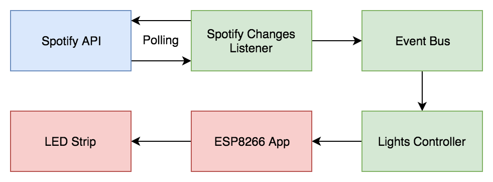
The app is fairly simple and essentially consists of two asyncio coroutines and a queue as a messaging bus.

The first coroutine calls Spotify API current playing endpoint, fetches audio analysis when the current playing song changes and produces three events:

  • EventStop – nothing is playing;
  • EventSongChanged(analysis, start_time) – song changed;
  • EventAdjustStartTime(start_time) – sync song start time in case of discrepancies or manual changes.
async def _listen_to_spotify_changes(session: aiohttp.ClientSession) -> AsyncIterable[Event]:
    current_id = None
    while True:
        request_time = time.time()
        current = await _get_current_playing(session)
        if not current['is_playing']:
            current_id = None
            yield EventStop()
        elif current['item']['id'] != current_id:
            current_id = current['item']['id']
            analysis = await _get_audio_analysis(session, current_id)
            yield EventSongChanged(analysis, _get_start_time(current, request_time))
        else:
            yield EventAdjustStartTime(_get_start_time(current, request_time))

        await asyncio.sleep(SPOTIFY_CHANGES_LISTENER_DEALY)


async def spotify_changes_listener(user_id: str,
                                   client_id: str,
                                   client_secret: str,
                                   events_queue: asyncio.Queue[Event]) -> NoReturn:
    while True:
        ...
        async with aiohttp.ClientSession(headers=headers) as session:
            try:
                async for event in _listen_to_spotify_changes(session):
                    await events_queue.put(event)
            except Exception:
                logging.exception('Something went wrong with spotify_changes_listener')

                await asyncio.sleep(SPOTIFY_CHANGES_LISTENER_FAILURE_DELAY)

The second coroutine listens to those events and sends packets to ESP8266:

async def lights_controller(device_ip: str,
                            device_port: int,
                            leds: int,
                            events_queue: asyncio.Queue[Event]) -> NoReturn:
    while True:
        send_to_device = await make_send_to_device(device_ip, device_port)
        try:
            async for colors in _events_to_colors(leds, events_queue):
                send_to_device(colors)

        except Exception:
            logging.exception("Something went wrong with lights_controller")
            await asyncio.sleep(CONTROLLER_ERROR_DELAY)

Full source code is a bit boring and available in the gist, to use it you will need to define some required environment variables.

The result

It works, kind of reusable and even looks a bit nice in real life, but not so nice when recorded on my phone:

Gist with everything.

Analysing music habits with Spotify API and Python


Hero image

I’m using Spotify since 2013 as the main source of music, and back at that time the app automatically created a playlist for songs that I liked from artists’ radios. By innertion I’m still using the playlist to save songs that I like. As the playlist became a bit big and a bit old (6 years, huh), I’ve decided to try to analyze it.

Boring preparation

To get the data I used Spotify API and spotipy as a Python client. I’ve created an application in the Spotify Dashboard and gathered the credentials. Then I was able to initialize and authorize the client:

import spotipy
import spotipy.util as util

token = util.prompt_for_user_token(user_id,
                                   'playlist-read-collaborative',
                                   client_id=client_id,
                                   client_secret=client_secret,
                                   redirect_uri='http://localhost:8000/')
sp = spotipy.Spotify(auth=token)

Tracks metadata

As everything is inside just one playlist, it was easy to gather. The only problem was that user_playlist method in spotipy doesn’t support pagination and can only return the first 100 track, but it was easily solved by just going down to private and undocumented _get:

playlist = sp.user_playlist(user_id, playlist_id)
tracks = playlist['tracks']['items']
next_uri = playlist['tracks']['next']
for _ in range(int(playlist['tracks']['total'] / playlist['tracks']['limit'])):
    response = sp._get(next_uri)
    tracks += response['items']
    next_uri = response['next']

tracks_df = pd.DataFrame([(track['track']['id'],
                           track['track']['artists'][0]['name'],
                           track['track']['name'],
                           parse_date(track['track']['album']['release_date']) if track['track']['album']['release_date'] else None,
                           parse_date(track['added_at']))
                          for track in playlist['tracks']['items']],
                         columns=['id', 'artist', 'name', 'release_date', 'added_at'] )
tracks_df.head(10)
id artist name release_date added_at
0 1MLtdVIDLdupSO1PzNNIQg Lindstrøm & Christabelle Looking For What 2009-12-11 2013-06-19 08:28:56+00:00
1 1gWsh0T1gi55K45TMGZxT0 Au Revoir Simone Knight Of Wands - Dam Mantle Remix 2010-07-04 2013-06-19 08:48:30+00:00
2 0LE3YWM0W9OWputCB8Z3qt Fever Ray When I Grow Up - D. Lissvik Version 2010-10-02 2013-06-19 22:09:15+00:00
3 5FyiyLzbZt41IpWyMuiiQy Holy Ghost! Dumb Disco Ideas 2013-05-14 2013-06-19 22:12:42+00:00
4 5cgfva649kw89xznFpWCFd Nouvelle Vague Too Drunk To Fuck 2004-11-01 2013-06-19 22:22:54+00:00
5 3IVc3QK63DngBdW7eVker2 TR/ST F.T.F. 2012-11-16 2013-06-20 11:50:58+00:00
6 0mbpEDdZHNMEDll6woEy8W Art Brut My Little Brother 2005-10-02 2013-06-20 13:58:19+00:00
7 2y8IhUDSpvsuuEePNLjGg5 Niki & The Dove Somebody (drum machine version) 2011-06-14 2013-06-21 09:28:40+00:00
8 1X4RqFAShNL8aHfUIpjIVr Gorillaz Kids with Guns - Hot Chip Remix 2007-11-19 2013-06-23 19:00:57+00:00
9 1cV4DVeAM5AstrDlXgvzJ7 Lykke Li I'm Good, I'm Gone 2008-01-28 2013-06-23 22:31:52+00:00

The first naive idea of data to get was the list of the most appearing artists:

tracks_df \
    .groupby('artist') \
    .count()['id'] \
    .reset_index() \
    .sort_values('id', ascending=False) \
    .rename(columns={'id': 'amount'}) \
    .head(10)
artist amount
260 Pet Shop Boys 12
334 The Knife 11
213 Metronomy 9
303 Soulwax 8
284 Röyksopp 7
180 Ladytron 7
94 Depeche Mode 7
113 Fever Ray 6
324 The Chemical Brothers 6
233 New Order 6

But as taste can change, I’ve decided to get top five artists from each year and check if I was adding them to the playlist in other years:

counted_year_df = tracks_df \
    .assign(year_added=tracks_df.added_at.dt.year) \
    .groupby(['artist', 'year_added']) \
    .count()['id'] \
    .reset_index() \
    .rename(columns={'id': 'amount'}) \
    .sort_values('amount', ascending=False)

in_top_5_year_artist = counted_year_df \
    .groupby('year_added') \
    .head(5) \
    .artist \
    .unique()

counted_year_df \
    [counted_year_df.artist.isin(in_top_5_year_artist)] \
    .pivot('artist', 'year_added', 'amount') \
    .fillna(0) \
    .style.background_gradient()
year_added 2013 2014 2015 2016 2017 2018 2019
artist
Arcade Fire 2 0 0 1 3 0 0
Clinic 1 0 0 2 0 0 1
Crystal Castles 0 0 2 2 0 0 0
Depeche Mode 1 0 3 1 0 2 0
Die Antwoord 1 4 0 0 0 1 0
FM Belfast 3 3 0 0 0 0 0
Factory Floor 3 0 0 0 0 0 0
Fever Ray 3 1 1 0 1 0 0
Grimes 1 0 3 1 0 0 0
Holy Ghost! 1 0 0 0 3 1 1
Joe Goddard 0 0 0 0 3 1 0
John Maus 0 0 4 0 0 0 1
KOMPROMAT 0 0 0 0 0 0 2
LCD Soundsystem 0 0 1 0 3 0 0
Ladytron 5 1 0 0 0 1 0
Lindstrøm 0 0 0 0 0 0 2
Marie Davidson 0 0 0 0 0 0 2
Metronomy 0 1 0 6 0 1 1
Midnight Magic 0 4 0 0 1 0 0
Mr. Oizo 0 0 0 1 0 3 0
New Order 1 5 0 0 0 0 0
Pet Shop Boys 0 12 0 0 0 0 0
Röyksopp 0 4 0 3 0 0 0
Schwefelgelb 0 0 0 0 1 0 4
Soulwax 0 0 0 0 5 3 0
Talking Heads 0 0 3 0 0 0 0
The Chemical Brothers 0 0 2 0 1 0 3
The Fall 0 0 0 0 0 2 0
The Knife 5 1 3 1 0 0 1
The Normal 0 0 0 2 0 0 0
The Prodigy 0 0 0 0 0 2 0
Vitalic 0 0 0 0 2 2 0

As a bunch of artists was reappearing in different years, I decided to check if that correlates with new releases, so I’ve checked the last ten years:

counted_release_year_df = tracks_df \
    .assign(year_added=tracks_df.added_at.dt.year,
            year_released=tracks_df.release_date.dt.year) \
    .groupby(['year_released', 'year_added']) \
    .count()['id'] \
    .reset_index() \
    .rename(columns={'id': 'amount'}) \
    .sort_values('amount', ascending=False)

counted_release_year_df \
    [counted_release_year_df.year_released.isin(
        sorted(tracks_df.release_date.dt.year.unique())[-11:]
    )] \
    .pivot('year_released', 'year_added', 'amount') \
    .fillna(0) \
    .style.background_gradient()
year_added 2013 2014 2015 2016 2017 2018 2019
year_released
2010.0 19 8 2 10 6 5 10
2011.0 14 10 4 6 5 5 5
2012.0 11 15 6 5 8 2 0
2013.0 28 17 3 6 5 4 2
2014.0 0 30 2 1 0 10 1
2015.0 0 0 15 5 8 7 9
2016.0 0 0 0 8 7 4 5
2017.0 0 0 0 0 23 5 5
2018.0 0 0 0 0 0 4 8
2019.0 0 0 0 0 0 0 14

Audio features

Spotify API has an endpoint that provides features like danceability, energy, loudness and etc for tracks. So I gathered features for all tracks from the playlist:

features = []
for n, chunk_series in tracks_df.groupby(np.arange(len(tracks_df)) // 50).id:
    features += sp.audio_features([*map(str, chunk_series)])
features_df = pd.DataFrame.from_dict(filter(None, features))
tracks_with_features_df = tracks_df.merge(features_df, on=['id'], how='inner')
tracks_with_features_df.head()
id artist name release_date added_at danceability energy key loudness mode speechiness acousticness instrumentalness liveness valence tempo duration_ms time_signature
0 1MLtdVIDLdupSO1PzNNIQg Lindstrøm & Christabelle Looking For What 2009-12-11 2013-06-19 08:28:56+00:00 0.566 0.726 0 -11.294 1 0.1120 0.04190 0.494000 0.282 0.345 120.055 359091 4
1 1gWsh0T1gi55K45TMGZxT0 Au Revoir Simone Knight Of Wands - Dam Mantle Remix 2010-07-04 2013-06-19 08:48:30+00:00 0.563 0.588 4 -7.205 0 0.0637 0.00573 0.932000 0.104 0.467 89.445 237387 4
2 0LE3YWM0W9OWputCB8Z3qt Fever Ray When I Grow Up - D. Lissvik Version 2010-10-02 2013-06-19 22:09:15+00:00 0.687 0.760 5 -6.236 1 0.0479 0.01160 0.007680 0.417 0.818 92.007 270120 4
3 5FyiyLzbZt41IpWyMuiiQy Holy Ghost! Dumb Disco Ideas 2013-05-14 2013-06-19 22:12:42+00:00 0.752 0.831 10 -4.407 1 0.0401 0.00327 0.729000 0.105 0.845 124.234 483707 4
4 5cgfva649kw89xznFpWCFd Nouvelle Vague Too Drunk To Fuck 2004-11-01 2013-06-19 22:22:54+00:00 0.461 0.786 7 -6.950 1 0.0467 0.47600 0.000003 0.495 0.808 159.882 136160 4

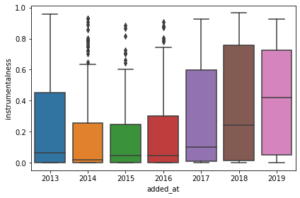
After that I’ve checked changes in features over time, only instrumentalness had some visible difference:

sns.boxplot(x=tracks_with_features_df.added_at.dt.year,
            y=tracks_with_features_df.instrumentalness)

Instrumentalness over time

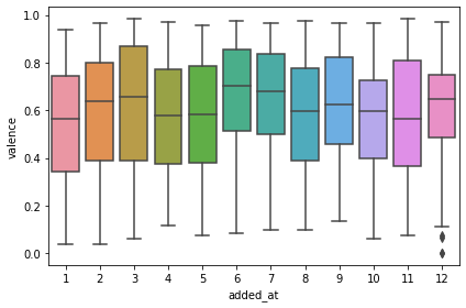
Then I had an idea to check seasonality and valence, and it kind of showed that in depressing months valence is a bit lower:

sns.boxplot(x=tracks_with_features_df.added_at.dt.month,
            y=tracks_with_features_df.valence)

Valence seasonality

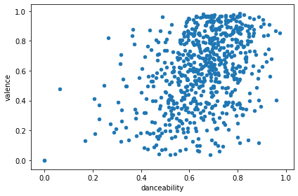
To play a bit more with data, I decided to check that danceability and valence might correlate:

tracks_with_features_df.plot(kind='scatter', x='danceability', y='valence')

Dnaceability vs valence

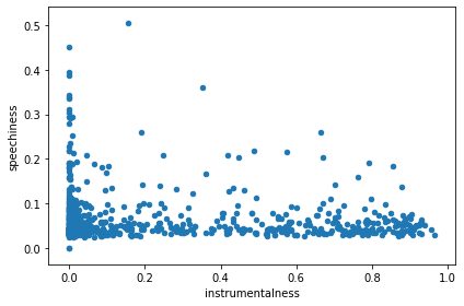
And to check that the data is meaningful, I checked instrumentalness vs speechiness, and those featues looked mutually exclusive as expected:

tracks_with_features_df.plot(kind='scatter', x='instrumentalness', y='speechiness')

Speachness vs instrumentalness

Tracks difference and similarity

As I already had a bunch of features classifying tracks, it was hard not to make vectors out of them:

encode_fields = [
    'danceability',
    'energy',
    'key',
    'loudness',
    'mode',
    'speechiness',
    'acousticness',
    'instrumentalness',
    'liveness',
    'valence',
    'tempo',
    'duration_ms',
    'time_signature',
]

def encode(row):
    return np.array([
        (row[k] - tracks_with_features_df[k].min())
        / (tracks_with_features_df[k].max() - tracks_with_features_df[k].min())
        for k in encode_fields])

tracks_with_features_encoded_df = tracks_with_features_df.assign(
    encoded=tracks_with_features_df.apply(encode, axis=1))

Then I just calculated distance between every two tracks:

tracks_with_features_encoded_product_df = tracks_with_features_encoded_df \
    .assign(temp=0) \
    .merge(tracks_with_features_encoded_df.assign(temp=0), on='temp', how='left') \
    .drop(columns='temp')
tracks_with_features_encoded_product_df = tracks_with_features_encoded_product_df[
    tracks_with_features_encoded_product_df.id_x != tracks_with_features_encoded_product_df.id_y
]
tracks_with_features_encoded_product_df['merge_id'] = tracks_with_features_encoded_product_df \
    .apply(lambda row: ''.join(sorted([row['id_x'], row['id_y']])), axis=1)
tracks_with_features_encoded_product_df['distance'] = tracks_with_features_encoded_product_df \
    .apply(lambda row: np.linalg.norm(row['encoded_x'] - row['encoded_y']), axis=1)

After that I was able to get most similar songs/songs with the minimal distance, and it selected kind of similar songs:

tracks_with_features_encoded_product_df \
    .sort_values('distance') \
    .drop_duplicates('merge_id') \
    [['artist_x', 'name_x', 'release_date_x', 'artist_y', 'name_y', 'release_date_y', 'distance']] \
    .head(10)
artist_x name_x release_date_x artist_y name_y release_date_y distance
84370 Labyrinth Ear Wild Flowers 2010-11-21 Labyrinth Ear Navy Light 2010-11-21 0.000000
446773 YACHT I Thought the Future Would Be Cooler 2015-09-11 ADULT. Love Lies 2013-05-13 0.111393
21963 Ladytron Seventeen 2011-03-29 The Juan Maclean Give Me Every Little Thing 2005-07-04 0.125358
11480 Class Actress Careful What You Say 2010-02-09 MGMT Little Dark Age 2017-10-17 0.128865
261780 Queen of Japan I Was Made For Loving You 2001-10-02 Midnight Juggernauts Devil Within 2007-10-02 0.131304
63257 Pixies Bagboy 2013-09-09 Kindness That's Alright 2012-03-16 0.146897
265792 Datarock Computer Camp Love 2005-10-02 Chromeo Night By Night 2010-09-21 0.147235
75359 Midnight Juggernauts Devil Within 2007-10-02 Lykke Li I'm Good, I'm Gone 2008-01-28 0.152680
105246 ADULT. Love Lies 2013-05-13 Dr. Alban Sing Hallelujah! 1992-05-04 0.154475
285180 Gigamesh Don't Stop 2012-05-28 Pet Shop Boys Paninaro 95 - 2003 Remaster 2003-10-02 0.156469

The most different songs weren’t that fun, as two songs were too different from the rest:

tracks_with_features_encoded_product_df \
    .sort_values('distance', ascending=False) \
    .drop_duplicates('merge_id') \
    [['artist_x', 'name_x', 'release_date_x', 'artist_y', 'name_y', 'release_date_y', 'distance']] \
    .head(10)
artist_x name_x release_date_x artist_y name_y release_date_y distance
79324 Labyrinth Ear Navy Light 2010-11-21 Boy Harsher Modulations 2014-10-01 2.480206
84804 Labyrinth Ear Wild Flowers 2010-11-21 Boy Harsher Modulations 2014-10-01 2.480206
400840 Charlotte Gainsbourg Deadly Valentine - Soulwax Remix 2017-11-10 Labyrinth Ear Navy Light 2010-11-21 2.478183
84840 Labyrinth Ear Wild Flowers 2010-11-21 Charlotte Gainsbourg Deadly Valentine - Soulwax Remix 2017-11-10 2.478183
388510 Ladytron Paco! 2001-10-02 Labyrinth Ear Navy Light 2010-11-21 2.444927
388518 Ladytron Paco! 2001-10-02 Labyrinth Ear Wild Flowers 2010-11-21 2.444927
20665 Factory Floor Fall Back 2013-01-15 Labyrinth Ear Navy Light 2010-11-21 2.439136
20673 Factory Floor Fall Back 2013-01-15 Labyrinth Ear Wild Flowers 2010-11-21 2.439136
79448 Labyrinth Ear Navy Light 2010-11-21 La Femme Runway 2018-10-01 2.423574
84928 Labyrinth Ear Wild Flowers 2010-11-21 La Femme Runway 2018-10-01 2.423574

Then I calculated the most avarage songs, eg the songs with the least distance from every other song:

tracks_with_features_encoded_product_df \
    .groupby(['artist_x', 'name_x', 'release_date_x']) \
    .sum()['distance'] \
    .reset_index() \
    .sort_values('distance') \
    .head(10)
artist_x name_x release_date_x distance
48 Beirut No Dice 2009-02-17 638.331257
591 The Juan McLean A Place Called Space 2014-09-15 643.436523
347 MGMT Little Dark Age 2017-10-17 645.959770
101 Class Actress Careful What You Say 2010-02-09 646.488998
31 Architecture In Helsinki 2 Time 2014-04-01 648.692344
588 The Juan Maclean Give Me Every Little Thing 2005-07-04 648.878463
323 Lindstrøm Baby Can't Stop 2009-10-26 652.212858
307 Ladytron Seventeen 2011-03-29 652.759843
310 Lauer Mirrors (feat. Jasnau) 2018-11-16 655.498535
451 Pet Shop Boys Always on My Mind 1998-03-31 656.437048

And totally opposite thing – the most outstanding songs:

tracks_with_features_encoded_product_df \
    .groupby(['artist_x', 'name_x', 'release_date_x']) \
    .sum()['distance'] \
    .reset_index() \
    .sort_values('distance', ascending=False) \
    .head(10)
artist_x name_x release_date_x distance
665 YACHT Le Goudron - Long Version 2012-05-25 2823.572387
300 Labyrinth Ear Navy Light 2010-11-21 1329.234390
301 Labyrinth Ear Wild Flowers 2010-11-21 1329.234390
57 Blonde Redhead For the Damaged Coda 2000-06-06 1095.393120
616 The Velvet Underground After Hours 1969-03-02 1080.491779
593 The Knife Forest Families 2006-02-17 1040.114214
615 The Space Lady Major Tom 2013-11-18 1016.881467
107 CocoRosie By Your Side 2004-03-09 1015.970860
170 El Perro Del Mar Party 2015-02-13 1012.163212
403 Mr.Kitty XIII 2014-10-06 1010.115117

Conclusion

Although the dataset is a bit small, it was still fun to have a look at the data.

Gist with a jupyter notebook with even more boring stuff, can be reused by modifying credentials.

Michael T. Nygard: Release It!


book cover white Not so long ago I’ve decided to read Release It! by Michael T. Nygard, and it’s a really awesome book. It covers all technical parts software development process from initial design, and planning to deployment, operations and possible inevitable failures. The book has a bunch of anti-patterns with fun to read case studies when everything went bad, but sometimes eventually resolved. It also covers good approaches with examples, but without going to “silver bullet” world.

One of the best books that I’ve recently read.

Robert C. Martin: Clean Architecture


book cover Recently I decided to read Clean Architecture by Robert C. Martin as I’m still trying to read something about system architecture and I had a good experience with Clean books in the past. And I kind of enjoyed it.

The book is about software architecture in general but mostly focused on “one piece of software” architecture. It nicely explains a few ways of proper separation of an application into different independent parts without going too deep into enterprise-ish practices and patterns. The book also shows a bunch of examples of how to abstract away implementation details, but also warns to not overdo and not over-engineer things.

Although sometimes it feels too basic and covers a lot of general knowledge, it’s a nice and useful book to read.

Mixing React Hooks with classes or making functional components more structured


Hook inside a class*

Relatively not so long ago Hooks were introduced in React. They allow us to have decoupled and reusable logic for components state and effects, and make dependency injection easier. But API wise it looks a bit like a step back from class-based components to sort of jQuery territory with tons of nested functions.

So I thought that it might be nice to try to mix both approaches.

TLDR: it’s possible to make it nice and declarative, but it requires metaprogramming and wouldn’t work in some browsers.

The hookable class adventure

Let’s assume that we have a simple counter component:

export default ({ initialCount }) => {
  const theme = useContext(Theme);

  const [current, setCurrent] = useState(initialCount);
  const [clicked, setClicked] = useState();

  const onClick = useCallback(() => {
    setCurrent(current + 1);
    setClicked(true);
  }, [current]);

  useEffect(() => {
    console.log("did mount");

    return () => {
      console.log("did unmount");
    };
  });

  return (
    <div>
      <p>
        Value: <span style=>{current}</span>
      </p>
      {clicked && <p>You already clicked!</p>}
      <p>Initial value: {initialCount}</p>
      <button onClick={onClick}>Increase</button>
    </div>
  );
};

As a first step towards classes, I made a simple decorator, that creates a function that initializes a class and calls render (the only similarity with original class-based components interfaces) method.

const asFunctional = cls => props => new cls(props).render();

As we can initialize attributes on a class body, it’s already safe to move useContext to it:

class Counter {
  theme = useContext(Theme);

  constructor({ initialCount }) {
    this.initialCount = initialCount;
  }

  render() {
    const [current, setCurrent] = useState(this.initialCount);
    const [clicked, setClicked] = useState();

    const onClick = useCallback(() => {
      setCurrent(current + 1);
      setClicked(true);
    }, [current]);

    useEffect(() => {
      console.log("did mount");

      return () => {
        console.log("did unmount");
      };
    });

    return (
      <div>
        <p>
          Value: <span style=>{current}</span>
        </p>
        {clicked && <p>You already clicked!</p>}
        <p>Initial value: {this.initialCount}</p>
        <button onClick={onClick}>Increase</button>
      </div>
    );
  }
}

export default asFunctional(Counter);

Manual assignment of props as attributes looks ugly, and useState inside render is even worse. It would be nice to be able to declare them on the class body. Unfortunately, decorators that can help with that aren’t here yet, but we can use a bit of Proxy magic by making a base class that will intercept attributes assignment and inject values for props and descriptors for the state:

const prop = () => ({ __isPropGetter: true });

const asDescriptor = ([val, setVal]) => ({
  __isDescriptor: true,
  get: () => val,
  set: newVal => setVal(newVal),
});

const Hookable = function(props) {
  return new Proxy(this, {
    set: (obj, name, val) => {
      if (val && val.__isPropGetter) {
        obj[name] = props[name];
      } else if (val && val.__isDescriptor) {
        Object.defineProperty(obj, name, val);
      } else {
        obj[name] = val;
      }
      return true;
    },
  });
};

So now we can have descriptors for the state, and when a state attribute value will be changed, set... will be called automatically. As we don’t need to have the state in a closure, it’s safe to move onClick callback to the class body:

class Counter extends Hookable {
  initialCount = prop();

  theme = useContext(Theme);

  current = asDescriptor(useState(this.initialCount));
  clicked = asDescriptor(useState());

  onClick = useCallback(() => {
    this.current += 1;
    this.clicked = true;
  }, [this.current]);

  render() {
    useEffect(() => {
      console.log("did mount");

      return () => {
        console.log("did unmount");
      };
    });

    return (
      <div>
        <p>
          Value: <span style=>{this.current}</span>
        </p>
        {this.clicked && <p>You already clicked!</p>}
        <p>Initial value: {this.initialCount}</p>
        <button onClick={this.onClick}>Increase</button>
      </div>
    );
  }
}

export default asFunctional(Counter);

The only not so fancy part left is useEffect inside render. In Python world similar problem with context managers API solved by contextmanager decorator, that transforms generators to context managers. I tried the same approach with effects:

const fromGenerator = (hook, genFn, deps) => fn => {
  const gen = genFn();
  hook(() => {
    gen.next();

    return () => {
      gen.next();
    };
  }, deps);

  return fn;
};

The magical end result

As a result, we have render with only JSX and almost no nested functions in our component:

class Counter extends Hookable {
  initialCount = prop();

  theme = useContext(Theme);

  current = asDescriptor(useState(this.initialCount));
  clicked = asDescriptor(useState());

  onClick = useCallback(() => {
    this.current += 1;
    this.clicked = true;
  }, [this.current]);

  withLogging = fromGenerator(
    useEffect,
    function*() {
      console.log("did mount");
      yield;
      console.log("did unmount");
    },
    [],
  );

  render = this.withLogging(() => (
    <div>
      <p>
        Value:{" "}
        <span style=>{this.current}</span>
      </p>
      {this.clicked && <p>You already clicked!</p>}
      <p>Initial value: {this.initialCount}</p>
      <button onClick={this.onClick}>Increase</button>
    </div>
  ));
}

export default asFunctional(Counter);

And it even works:

For my personal eyes, the end result looks better and more readable, but the magic inside isn’t free:

  • it doesn’t work in Internet Explorer
  • the machinery around Proxy might be slow
  • it’s impossible to make it properly typed with TypeScript or Flow
  • metaprogramming could make things unnecessary more complicated

So I guess something in the middle (functor-like approach?) might be useful for real applications.

Gist with source code.

* hero image contains a photo of a classroom in Alaska

Eben Hewitt: Technology Strategy Patterns


book cover white Not so long ago I wanted to read something about a large scale architecture and mistakenly decided that Technology Strategy Patterns by Eben Hewitt was about that. It’s not, but it was still interesting to read. The book provides a bunch of nice patterns for delivering information to product-people and stakeholders. The book covers a few ways of doing long-range planning and analysis with some examples from the real world. It even has some Powerpoint and Excel advice.

Although somehow the book was useful for me and I’ve learned a bunch of new stuff, I’m definitely not the target audience of it.

Finding the cheapest flights for a multi-leg trip with Amadeus API and Python


An old plane

This summer I’m planning to have a trip that will include Moscow, Irkutsk, Beijing, Shanghai, and Tokyo. As I’m flexible on dates I’ve decided to try to find the cheapest flights with the shortest duration. I’ve tried to do this before twice by parsing Google Flights, it was successful, but I don’t want to update those hackish scripts and want to try something a bit saner.

So I chose to try Amadeus API. It was a bit painful to use, some endpoints were randomly failing with 500, and they needed a signed agreement to use real data. But overall it was at least better than parsing Google Flights, and the whole adventure fit inside the free quota for requests.

TLDR: jupyter notebook with the whole adventure

Restrictions

I’m flexible but with boundaries, so I’ll be able to start between 10th and 20th of July and travel no longer than 21 days:

min_start = date(2019, 7, 10)
max_start = date(2019, 7, 20)
max_days = 21

I mostly don’t want to have multi-segment flights and know how many days I want to spend in destinations:

places_df = pd.DataFrame([('Amsterdam', 'NL', 0, (max_start - min_start).days, True),  # for enabling tentative start date
                          ('Moscow', 'RU', 3, 5, True),
                          ('Irkutsk', 'RU', 7, 10, True),
                          ('Beijing', 'CN', 3, 5, True),
                          ('Shanghai', 'CN', 3, 5, True),
                          ('Tokyo', 'JP', 3, 5, False),
                          ('Amsterdam', 'NL', 0, 0, True)],  # the final destination
                         columns=['city', 'cc', 'min_days', 'max_days', 'only_direct'])

places_df['min_day_of_dep'] = places_df.min_days.rolling(min_periods=1, window=len(places_df)).sum()
places_df['max_day_of_dep'] = places_df.max_days.rolling(min_periods=1, window=len(places_df)).sum()

places_df
city cc min_days max_days only_direct min_day_of_dep max_day_of_dep
0 Amsterdam NL 0 10 True 0.0 10.0
1 Moscow RU 3 5 True 3.0 15.0
2 Irkutsk RU 7 10 True 10.0 25.0
3 Beijing CN 3 5 True 13.0 30.0
4 Shanghai CN 3 5 True 16.0 35.0
5 Tokyo JP 3 5 False 19.0 40.0
6 Amsterdam NL 0 0 True 19.0 40.0

Airports

A lot of big cities have more than one airport, and usually, some airports are for low-costers and some for pricier flights. But the most important that the API expects me to send IATA codes to get prices for dates. So I needed to get IATA codes for airports for cities I will travel through, and it’s possible with just a request to /reference-data/locations:

def get_iata(city, cc):
    response = call_api('/reference-data/locations',  # full code in the notebook
                        keyword=city,
                        countryCode=cc,
                        subType='AIRPORT')

    return [result['iataCode'] for result in response['data']]

get_iata('Moscow', 'RU')
['DME', 'SVO', 'VKO']

With that function, I was able to get IATA codes for all destinations and get all possible routes with a bit of pandas magic:

places_df['iata'] = places_df.apply(lambda place: get_iata(place['city'], place['cc']), axis=1)

routes_df = places_df.assign(dest_iata=places_df.iloc[1:].reset_index().iata)
routes_df['routes'] = routes_df.apply(
    lambda row: [*product(row['iata'], row['dest_iata'])] if isinstance(row['dest_iata'], list) else [],
    axis=1)

routes_df = routes_df.routes \
    .apply(pd.Series) \
    .merge(routes_df, right_index=True, left_index=True) \
    .drop(['routes', 'min_days', 'max_days', 'iata', 'dest_iata'], axis=1) \
    .melt(id_vars=['city', 'cc', 'min_day_of_dep', 'max_day_of_dep', 'only_direct'], value_name="route") \
    .drop('variable', axis=1) \
    .dropna()

routes_df['origin'] = routes_df.route.apply(lambda route: route[0])
routes_df['destination'] = routes_df.route.apply(lambda route: route[1])
routes_df = routes_df \
    .drop('route', axis=1) \
    .rename(columns={'city': 'origin_city',
                     'cc': 'origin_cc'})

routes_df.head(10)
origin_city origin_cc min_day_of_dep max_day_of_dep only_direct origin destination
0 Amsterdam NL 0.0 10.0 True AMS DME
1 Moscow RU 3.0 15.0 True DME IKT
2 Irkutsk RU 10.0 25.0 True IKT PEK
3 Beijing CN 13.0 30.0 True PEK PVG
4 Shanghai CN 16.0 35.0 True PVG HND
5 Tokyo JP 19.0 40.0 False HND AMS
7 Amsterdam NL 0.0 10.0 True AMS SVO
8 Moscow RU 3.0 15.0 True SVO IKT
9 Irkutsk RU 10.0 25.0 True IKT NAY
10 Beijing CN 13.0 30.0 True PEK SHA

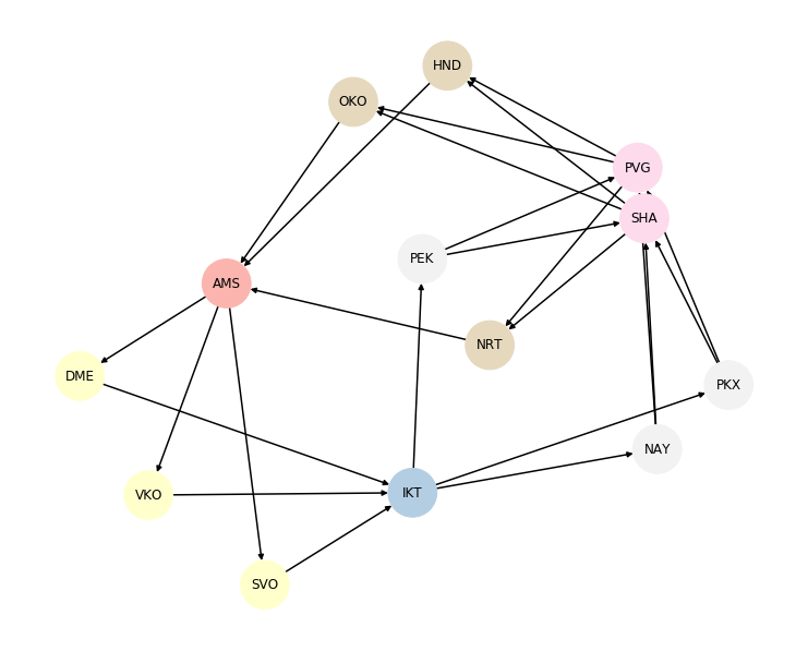
To understand the complexity of the problem better I draw an ugly graph of possible flights routes:

The ugly graph with airports

Prices and dates

After that I’ve calculated all possible dates for flights:

route_dates_df = routes_df.assign(
    dates=routes_df.apply(lambda row: [min_start + timedelta(days=days)
                                       for days in range(int(row.min_day_of_dep), int(row.max_day_of_dep) + 1)],
                          axis=1))

route_dates_df = route_dates_df.dates \
    .apply(pd.Series) \
    .merge(route_dates_df, right_index=True, left_index=True) \
    .drop(['dates', 'min_day_of_dep', 'max_day_of_dep'], axis=1) \
    .melt(id_vars=['origin_city', 'origin_cc', 'origin', 'destination', 'only_direct'], value_name="date") \
    .drop('variable', axis=1) \
    .dropna()

valid_routes_df = route_dates_df[route_dates_df.date <= max_start + timedelta(days=max_days)]

valid_routes_df.head(10)
origin_city origin_cc origin destination only_direct date
0 Amsterdam NL AMS DME True 2019-07-10
1 Moscow RU DME IKT True 2019-07-13
2 Irkutsk RU IKT PEK True 2019-07-20
3 Beijing CN PEK PVG True 2019-07-23
4 Shanghai CN PVG HND True 2019-07-26
5 Tokyo JP HND AMS False 2019-07-29
6 Amsterdam NL AMS SVO True 2019-07-10
7 Moscow RU SVO IKT True 2019-07-13
8 Irkutsk RU IKT NAY True 2019-07-20
9 Beijing CN PEK SHA True 2019-07-23

Eventually, I’ve got 363 possible route-date combinations, and used /shopping/flight-offers to get prices. As the endpoint has a quota of 2000 free requests, I was able to mess everything up a few times and haven’t reached it yet:

def get_prices(origin, destination, date, only_direct):
    response = call_api('/shopping/flight-offers',
                         origin=origin,
                         destination=destination,
                         nonStop='true' if only_direct else 'false',
                         departureDate=date.strftime("%Y-%m-%d"))

    if 'data' not in response:
        print(response)
        return []

    return [(origin, destination, date,
             Decimal(offer_item['price']['total']),
             parse_date(offer_item['services'][0]['segments'][0]['flightSegment']['departure']['at']),
             parse_date(offer_item['services'][0]['segments'][-1]['flightSegment']['arrival']['at']),
             len(offer_item['services'][0]['segments']))
            for flight in response['data']
            for offer_item in flight['offerItems']]

get_prices('IKT', 'PEK', date(2019, 7, 20), True)[:5]
[('IKT',
  'PEK',
  datetime.date(2019, 7, 20),
  Decimal('209.11'),
  datetime.datetime(2019, 7, 20, 1, 50, tzinfo=tzoffset(None, 28800)),
  datetime.datetime(2019, 7, 20, 4, 40, tzinfo=tzoffset(None, 28800)),
  1),
 ('IKT',
  'PEK',
  datetime.date(2019, 7, 20),
  Decimal('262.98'),
  datetime.datetime(2019, 7, 20, 15, 15, tzinfo=tzoffset(None, 28800)),
  datetime.datetime(2019, 7, 20, 18, 5, tzinfo=tzoffset(None, 28800)),
  1)]

Then I’ve fetched flights for the whole set of dates, assigned useful metadata like origin/destination cities and duration of the flights, and removed flights pricier than €800:

prices_df = pd.DataFrame([price
                          for route in valid_routes_df.to_dict('record')
                          for price in get_prices(route['origin'], route['destination'], route['date'], route['only_direct'])],
                         columns=['origin', 'destination', 'date', 'price', 'departure_at', 'arrival_at', 'segments'])

airport_to_city = dict(zip(routes_df.origin, routes_df.origin_city))

prices_with_city_df = prices_df \
    .assign(duration=prices_df.arrival_at - prices_df.departure_at,
            origin_city=prices_df.origin.apply(airport_to_city.__getitem__),
            destination_city=prices_df.destination.apply(airport_to_city.__getitem__))
prices_with_city_df['route'] = prices_with_city_df.origin_city + " ✈️ " + prices_with_city_df.destination_city

valid_prices_with_city_df = prices_with_city_df[prices_with_city_df.price <= 800]

valid_prices_with_city_df.head()
origin destination date price departure_at arrival_at segments duration origin_city destination_city route
0 DME IKT 2019-07-13 257.40 2019-07-13 21:40:00+03:00 2019-07-14 08:25:00+08:00 1 05:45:00 Moscow Irkutsk Moscow✈️Irkutsk
1 DME IKT 2019-07-13 257.40 2019-07-13 23:00:00+03:00 2019-07-14 09:45:00+08:00 1 05:45:00 Moscow Irkutsk Moscow✈️Irkutsk
2 DME IKT 2019-07-13 254.32 2019-07-13 19:55:00+03:00 2019-07-14 06:25:00+08:00 1 05:30:00 Moscow Irkutsk Moscow✈️Irkutsk
3 DME IKT 2019-07-13 227.40 2019-07-13 18:30:00+03:00 2019-07-14 05:15:00+08:00 1 05:45:00 Moscow Irkutsk Moscow✈️Irkutsk
4 IKT PEK 2019-07-20 209.11 2019-07-20 01:50:00+08:00 2019-07-20 04:40:00+08:00 1 02:50:00 Irkutsk Beijing Irkutsk✈️Beijing

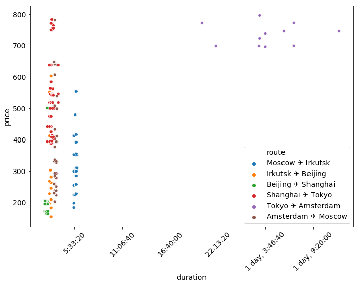
To have a brief overview of prices I’ve made a scatterplot. If I was a machine learning algorithm I would exclude Tokyo from the adventure:

Scatterplot with prices and duration

Itinerary

At this stage I’ve got all the data I want, so I can begin building the itinerary. I’ve calculated all possible city/date combination of flights. Job interviews questions prepared me for that:

next_flight_origin_city = dict(zip(places_df.city.iloc[:-2], places_df.city.iloc[1:-1]))
place_min_days = dict(zip(places_df.city.iloc[:-1], places_df.min_days.iloc[:-1]))
place_max_days = dict(zip(places_df.city.iloc[:-1], places_df.max_days.iloc[:-1]))

def build_itinerary(place, date):
    if place is None:
        return

    next_place = next_flight_origin_city.get(place)

    for days in range(place_min_days[place], place_max_days[place] + 1):
        flight_date = date + timedelta(days=days)
        for rest_flights in build_itinerary(next_place, flight_date):
            yield [(place, flight_date), *rest_flights]

        if next_place is None:
            yield [(place, flight_date)]

itinerary = [*build_itinerary('Amsterdam', min_start)]
itinerary[:3]
[[('Amsterdam', datetime.date(2019, 7, 10)),
  ('Moscow', datetime.date(2019, 7, 13)),
  ('Irkutsk', datetime.date(2019, 7, 20)),
  ('Beijing', datetime.date(2019, 7, 23)),
  ('Shanghai', datetime.date(2019, 7, 26)),
  ('Tokyo', datetime.date(2019, 7, 29))],
 [('Amsterdam', datetime.date(2019, 7, 10)),
  ('Moscow', datetime.date(2019, 7, 13)),
  ('Irkutsk', datetime.date(2019, 7, 20)),
  ('Beijing', datetime.date(2019, 7, 23)),
  ('Shanghai', datetime.date(2019, 7, 26)),
  ('Tokyo', datetime.date(2019, 7, 30))],
 [('Amsterdam', datetime.date(2019, 7, 10)),
  ('Moscow', datetime.date(2019, 7, 13)),
  ('Irkutsk', datetime.date(2019, 7, 20)),
  ('Beijing', datetime.date(2019, 7, 23)),
  ('Shanghai', datetime.date(2019, 7, 26)),
  ('Tokyo', datetime.date(2019, 7, 31))]]

And then I’ve found all flights for those dates. As amount of possible flights combinations didn’t fit in my RAM, I was selecting n_cheapest flights on each stage. The code is slow and ugly, but it worked:

def find_flights(prices_with_city_df, itinerary_route, n_cheapest):
    result_df = None
    for place, date in itinerary_route:
        place_df = prices_with_city_df \
            [(prices_with_city_df.origin_city == place) & (prices_with_city_df.date == date)] \
            .sort_values('price', ascending=True) \
            .head(n_cheapest) \
            .add_prefix(f'{place}_')

        if result_df is None:
            result_df = place_df
        else:
            result_df = result_df \
                .assign(key=1) \
                .merge(place_df.assign(key=1), on="key") \
                .drop("key", axis=1)

            result_df['total_price'] = reduce(operator.add, (
                result_df[column] for column in result_df.columns
                if 'price' in column and column != 'total_price'
            ))

            result_df = result_df \
                .sort_values('total_price', ascending=True) \
                .head(n_cheapest)

    result_df['total_flights_duration'] = reduce(operator.add, (
        result_df[column] for column in result_df.columns
        if 'duration' in column
    ))

    return result_df[['total_price', 'total_flights_duration'] + [
        column for column in result_df.columns
        if 'total_' not in column]]

find_flights(prices_with_city_df, itinerary[0], 100).head(5)
total_price total_flights_duration Amsterdam_origin Amsterdam_destination Amsterdam_date Amsterdam_price Amsterdam_departure_at Amsterdam_arrival_at Amsterdam_segments Amsterdam_duration Amsterdam_origin_city Amsterdam_destination_city Amsterdam_route Moscow_origin Moscow_destination Moscow_date Moscow_price Moscow_departure_at Moscow_arrival_at Moscow_segments Moscow_duration Moscow_origin_city Moscow_destination_city Moscow_route Irkutsk_origin Irkutsk_destination Irkutsk_date Irkutsk_price Irkutsk_departure_at Irkutsk_arrival_at Irkutsk_segments Irkutsk_duration Irkutsk_origin_city Irkutsk_destination_city Irkutsk_route Beijing_origin Beijing_destination Beijing_date Beijing_price Beijing_departure_at Beijing_arrival_at Beijing_segments Beijing_duration Beijing_origin_city Beijing_destination_city Beijing_route Shanghai_origin Shanghai_destination Shanghai_date Shanghai_price Shanghai_departure_at Shanghai_arrival_at Shanghai_segments Shanghai_duration Shanghai_origin_city Shanghai_destination_city Shanghai_route Tokyo_origin Tokyo_destination Tokyo_date Tokyo_price Tokyo_departure_at Tokyo_arrival_at Tokyo_segments Tokyo_duration Tokyo_origin_city Tokyo_destination_city Tokyo_route
0 1901.41 1 days 20:45:00 AMS SVO 2019-07-10 203.07 2019-07-10 21:15:00+02:00 2019-07-11 01:30:00+03:00 1 03:15:00 Amsterdam Moscow Amsterdam ✈️ Moscow DME IKT 2019-07-13 227.40 2019-07-13 18:30:00+03:00 2019-07-14 05:15:00+08:00 1 05:45:00 Moscow Irkutsk Moscow ✈️ Irkutsk IKT PEK 2019-07-20 209.11 2019-07-20 01:50:00+08:00 2019-07-20 04:40:00+08:00 1 02:50:00 Irkutsk Beijing Irkutsk ✈️ Beijing PEK SHA 2019-07-23 171.64 2019-07-23 11:30:00+08:00 2019-07-23 14:00:00+08:00 1 02:30:00 Beijing Shanghai Beijing ✈️ Shanghai SHA NRT 2019-07-26 394.07 2019-07-26 14:35:00+08:00 2019-07-26 18:15:00+09:00 1 02:40:00 Shanghai Tokyo Shanghai ✈️ Tokyo NRT AMS 2019-07-29 696.12 2019-07-29 17:55:00+09:00 2019-07-30 14:40:00+02:00 2 1 days 03:45:00 Tokyo Amsterdam Tokyo ✈️ Amsterdam
2800 1901.41 1 days 20:30:00 AMS SVO 2019-07-10 203.07 2019-07-10 11:50:00+02:00 2019-07-10 16:05:00+03:00 1 03:15:00 Amsterdam Moscow Amsterdam ✈️ Moscow DME IKT 2019-07-13 227.40 2019-07-13 18:30:00+03:00 2019-07-14 05:15:00+08:00 1 05:45:00 Moscow Irkutsk Moscow ✈️ Irkutsk IKT PEK 2019-07-20 209.11 2019-07-20 01:50:00+08:00 2019-07-20 04:40:00+08:00 1 02:50:00 Irkutsk Beijing Irkutsk ✈️ Beijing PEK SHA 2019-07-23 171.64 2019-07-23 21:30:00+08:00 2019-07-23 23:45:00+08:00 1 02:15:00 Beijing Shanghai Beijing ✈️ Shanghai PVG NRT 2019-07-26 394.07 2019-07-26 14:35:00+08:00 2019-07-26 18:15:00+09:00 1 02:40:00 Shanghai Tokyo Shanghai ✈️ Tokyo NRT AMS 2019-07-29 696.12 2019-07-29 17:55:00+09:00 2019-07-30 14:40:00+02:00 2 1 days 03:45:00 Tokyo Amsterdam Tokyo ✈️ Amsterdam
2900 1901.41 1 days 20:30:00 AMS SVO 2019-07-10 203.07 2019-07-10 21:15:00+02:00 2019-07-11 01:30:00+03:00 1 03:15:00 Amsterdam Moscow Amsterdam ✈️ Moscow DME IKT 2019-07-13 227.40 2019-07-13 18:30:00+03:00 2019-07-14 05:15:00+08:00 1 05:45:00 Moscow Irkutsk Moscow ✈️ Irkutsk IKT PEK 2019-07-20 209.11 2019-07-20 01:50:00+08:00 2019-07-20 04:40:00+08:00 1 02:50:00 Irkutsk Beijing Irkutsk ✈️ Beijing PEK SHA 2019-07-23 171.64 2019-07-23 10:00:00+08:00 2019-07-23 12:15:00+08:00 1 02:15:00 Beijing Shanghai Beijing ✈️ Shanghai SHA NRT 2019-07-26 394.07 2019-07-26 14:35:00+08:00 2019-07-26 18:15:00+09:00 1 02:40:00 Shanghai Tokyo Shanghai ✈️ Tokyo NRT AMS 2019-07-29 696.12 2019-07-29 17:55:00+09:00 2019-07-30 14:40:00+02:00 2 1 days 03:45:00 Tokyo Amsterdam Tokyo ✈️ Amsterdam
3000 1901.41 1 days 20:30:00 AMS SVO 2019-07-10 203.07 2019-07-10 21:15:00+02:00 2019-07-11 01:30:00+03:00 1 03:15:00 Amsterdam Moscow Amsterdam ✈️ Moscow DME IKT 2019-07-13 227.40 2019-07-13 18:30:00+03:00 2019-07-14 05:15:00+08:00 1 05:45:00 Moscow Irkutsk Moscow ✈️ Irkutsk IKT PEK 2019-07-20 209.11 2019-07-20 01:50:00+08:00 2019-07-20 04:40:00+08:00 1 02:50:00 Irkutsk Beijing Irkutsk ✈️ Beijing PEK SHA 2019-07-23 171.64 2019-07-23 10:00:00+08:00 2019-07-23 12:15:00+08:00 1 02:15:00 Beijing Shanghai Beijing ✈️ Shanghai PVG NRT 2019-07-26 394.07 2019-07-26 14:35:00+08:00 2019-07-26 18:15:00+09:00 1 02:40:00 Shanghai Tokyo Shanghai ✈️ Tokyo NRT AMS 2019-07-29 696.12 2019-07-29 17:55:00+09:00 2019-07-30 14:40:00+02:00 2 1 days 03:45:00 Tokyo Amsterdam Tokyo ✈️ Amsterdam
3100 1901.41 1 days 20:30:00 AMS SVO 2019-07-10 203.07 2019-07-10 21:15:00+02:00 2019-07-11 01:30:00+03:00 1 03:15:00 Amsterdam Moscow Amsterdam ✈️ Moscow DME IKT 2019-07-13 227.40 2019-07-13 18:30:00+03:00 2019-07-14 05:15:00+08:00 1 05:45:00 Moscow Irkutsk Moscow ✈️ Irkutsk IKT PEK 2019-07-20 209.11 2019-07-20 01:50:00+08:00 2019-07-20 04:40:00+08:00 1 02:50:00 Irkutsk Beijing Irkutsk ✈️ Beijing PEK SHA 2019-07-23 171.64 2019-07-23 17:00:00+08:00 2019-07-23 19:15:00+08:00 1 02:15:00 Beijing Shanghai Beijing ✈️ Shanghai SHA NRT 2019-07-26 394.07 2019-07-26 14:35:00+08:00 2019-07-26 18:15:00+09:00 1 02:40:00 Shanghai Tokyo Shanghai ✈️ Tokyo NRT AMS 2019-07-29 696.12 2019-07-29 17:55:00+09:00 2019-07-30 14:40:00+02:00 2 1 days 03:45:00 Tokyo Amsterdam Tokyo ✈️ Amsterdam

So now it’s easy to get the cheapest flights by calling the function for all possible itineraries:

itinerary_df = reduce(pd.DataFrame.append, (find_flights(prices_with_city_df, itinerary_route, 10)
                                           for itinerary_route in itinerary))

itinerary_df \
    .sort_values(['total_price', 'total_flights_duration']) \
    .head(10)
total_price total_flights_duration Amsterdam_origin Amsterdam_destination Amsterdam_date Amsterdam_price Amsterdam_departure_at Amsterdam_arrival_at Amsterdam_segments Amsterdam_duration Amsterdam_origin_city Amsterdam_destination_city Amsterdam_route Moscow_origin Moscow_destination Moscow_date Moscow_price Moscow_departure_at Moscow_arrival_at Moscow_segments Moscow_duration Moscow_origin_city Moscow_destination_city Moscow_route Irkutsk_origin Irkutsk_destination Irkutsk_date Irkutsk_price Irkutsk_departure_at Irkutsk_arrival_at Irkutsk_segments Irkutsk_duration Irkutsk_origin_city Irkutsk_destination_city Irkutsk_route Beijing_origin Beijing_destination Beijing_date Beijing_price Beijing_departure_at Beijing_arrival_at Beijing_segments Beijing_duration Beijing_origin_city Beijing_destination_city Beijing_route Shanghai_origin Shanghai_destination Shanghai_date Shanghai_price Shanghai_departure_at Shanghai_arrival_at Shanghai_segments Shanghai_duration Shanghai_origin_city Shanghai_destination_city Shanghai_route Tokyo_origin Tokyo_destination Tokyo_date Tokyo_price Tokyo_departure_at Tokyo_arrival_at Tokyo_segments Tokyo_duration Tokyo_origin_city Tokyo_destination_city Tokyo_route
10 1817.04 1 days 19:50:00 AMS SVO 2019-07-11 203.07 2019-07-11 21:15:00+02:00 2019-07-12 01:30:00+03:00 1 03:15:00 Amsterdam Moscow Amsterdam ✈️ Moscow DME IKT 2019-07-15 198.03 2019-07-15 18:35:00+03:00 2019-07-16 05:05:00+08:00 1 05:30:00 Moscow Irkutsk Moscow ✈️ Irkutsk IKT PEK 2019-07-22 154.11 2019-07-22 01:50:00+08:00 2019-07-22 04:40:00+08:00 1 02:50:00 Irkutsk Beijing Irkutsk ✈️ Beijing PEK SHA 2019-07-25 171.64 2019-07-25 21:50:00+08:00 2019-07-25 23:55:00+08:00 1 02:05:00 Beijing Shanghai Beijing ✈️ Shanghai PVG NRT 2019-07-28 394.07 2019-07-28 17:15:00+08:00 2019-07-28 20:40:00+09:00 1 02:25:00 Shanghai Tokyo Shanghai ✈️ Tokyo NRT AMS 2019-07-31 696.12 2019-07-31 17:55:00+09:00 2019-08-01 14:40:00+02:00 2 1 days 03:45:00 Tokyo Amsterdam Tokyo ✈️ Amsterdam
40 1817.04 1 days 19:50:00 AMS SVO 2019-07-11 203.07 2019-07-11 21:15:00+02:00 2019-07-12 01:30:00+03:00 1 03:15:00 Amsterdam Moscow Amsterdam ✈️ Moscow DME IKT 2019-07-15 198.03 2019-07-15 18:35:00+03:00 2019-07-16 05:05:00+08:00 1 05:30:00 Moscow Irkutsk Moscow ✈️ Irkutsk IKT PEK 2019-07-22 154.11 2019-07-22 01:50:00+08:00 2019-07-22 04:40:00+08:00 1 02:50:00 Irkutsk Beijing Irkutsk ✈️ Beijing PEK SHA 2019-07-25 171.64 2019-07-25 21:50:00+08:00 2019-07-25 23:55:00+08:00 1 02:05:00 Beijing Shanghai Beijing ✈️ Shanghai SHA NRT 2019-07-28 394.07 2019-07-28 17:15:00+08:00 2019-07-28 20:40:00+09:00 1 02:25:00 Shanghai Tokyo Shanghai ✈️ Tokyo NRT AMS 2019-07-31 696.12 2019-07-31 17:55:00+09:00 2019-08-01 14:40:00+02:00 2 1 days 03:45:00 Tokyo Amsterdam Tokyo ✈️ Amsterdam
0 1817.04 1 days 20:00:00 AMS SVO 2019-07-10 203.07 2019-07-10 21:15:00+02:00 2019-07-11 01:30:00+03:00 1 03:15:00 Amsterdam Moscow Amsterdam ✈️ Moscow DME IKT 2019-07-15 198.03 2019-07-15 18:35:00+03:00 2019-07-16 05:05:00+08:00 1 05:30:00 Moscow Irkutsk Moscow ✈️ Irkutsk IKT PEK 2019-07-22 154.11 2019-07-22 01:50:00+08:00 2019-07-22 04:40:00+08:00 1 02:50:00 Irkutsk Beijing Irkutsk ✈️ Beijing PEK SHA 2019-07-25 171.64 2019-07-25 13:00:00+08:00 2019-07-25 15:15:00+08:00 1 02:15:00 Beijing Shanghai Beijing ✈️ Shanghai PVG NRT 2019-07-28 394.07 2019-07-28 17:15:00+08:00 2019-07-28 20:40:00+09:00 1 02:25:00 Shanghai Tokyo Shanghai ✈️ Tokyo NRT AMS 2019-07-31 696.12 2019-07-31 17:55:00+09:00 2019-08-01 14:40:00+02:00 2 1 days 03:45:00 Tokyo Amsterdam Tokyo ✈️ Amsterdam
70 1817.04 1 days 20:00:00 AMS SVO 2019-07-10 203.07 2019-07-10 11:50:00+02:00 2019-07-10 16:05:00+03:00 1 03:15:00 Amsterdam Moscow Amsterdam ✈️ Moscow DME IKT 2019-07-15 198.03 2019-07-15 18:35:00+03:00 2019-07-16 05:05:00+08:00 1 05:30:00 Moscow Irkutsk Moscow ✈️ Irkutsk IKT PEK 2019-07-22 154.11 2019-07-22 01:50:00+08:00 2019-07-22 04:40:00+08:00 1 02:50:00 Irkutsk Beijing Irkutsk ✈️ Beijing PEK SHA 2019-07-25 171.64 2019-07-25 18:00:00+08:00 2019-07-25 20:15:00+08:00 1 02:15:00 Beijing Shanghai Beijing ✈️ Shanghai PVG NRT 2019-07-28 394.07 2019-07-28 17:15:00+08:00 2019-07-28 20:40:00+09:00 1 02:25:00 Shanghai Tokyo Shanghai ✈️ Tokyo NRT AMS 2019-07-31 696.12 2019-07-31 17:55:00+09:00 2019-08-01 14:40:00+02:00 2 1 days 03:45:00 Tokyo Amsterdam Tokyo ✈️ Amsterdam
60 1817.04 1 days 20:00:00 AMS SVO 2019-07-10 203.07 2019-07-10 11:50:00+02:00 2019-07-10 16:05:00+03:00 1 03:15:00 Amsterdam Moscow Amsterdam ✈️ Moscow DME IKT 2019-07-15 198.03 2019-07-15 18:35:00+03:00 2019-07-16 05:05:00+08:00 1 05:30:00 Moscow Irkutsk Moscow ✈️ Irkutsk IKT PEK 2019-07-22 154.11 2019-07-22 01:50:00+08:00 2019-07-22 04:40:00+08:00 1 02:50:00 Irkutsk Beijing Irkutsk ✈️ Beijing PEK SHA 2019-07-25 171.64 2019-07-25 13:00:00+08:00 2019-07-25 15:15:00+08:00 1 02:15:00 Beijing Shanghai Beijing ✈️ Shanghai PVG NRT 2019-07-28 394.07 2019-07-28 17:15:00+08:00 2019-07-28 20:40:00+09:00 1 02:25:00 Shanghai Tokyo Shanghai ✈️ Tokyo NRT AMS 2019-07-31 696.12 2019-07-31 17:55:00+09:00 2019-08-01 14:40:00+02:00 2 1 days 03:45:00 Tokyo Amsterdam Tokyo ✈️ Amsterdam
0 1817.04 1 days 20:00:00 AMS SVO 2019-07-11 203.07 2019-07-11 21:15:00+02:00 2019-07-12 01:30:00+03:00 1 03:15:00 Amsterdam Moscow Amsterdam ✈️ Moscow DME IKT 2019-07-15 198.03 2019-07-15 18:35:00+03:00 2019-07-16 05:05:00+08:00 1 05:30:00 Moscow Irkutsk Moscow ✈️ Irkutsk IKT PEK 2019-07-22 154.11 2019-07-22 01:50:00+08:00 2019-07-22 04:40:00+08:00 1 02:50:00 Irkutsk Beijing Irkutsk ✈️ Beijing PEK SHA 2019-07-25 171.64 2019-07-25 13:00:00+08:00 2019-07-25 15:15:00+08:00 1 02:15:00 Beijing Shanghai Beijing ✈️ Shanghai PVG NRT 2019-07-28 394.07 2019-07-28 17:15:00+08:00 2019-07-28 20:40:00+09:00 1 02:25:00 Shanghai Tokyo Shanghai ✈️ Tokyo NRT AMS 2019-07-31 696.12 2019-07-31 17:55:00+09:00 2019-08-01 14:40:00+02:00 2 1 days 03:45:00 Tokyo Amsterdam Tokyo ✈️ Amsterdam
10 1817.04 1 days 20:05:00 AMS SVO 2019-07-10 203.07 2019-07-10 11:50:00+02:00 2019-07-10 16:05:00+03:00 1 03:15:00 Amsterdam Moscow Amsterdam ✈️ Moscow DME IKT 2019-07-15 198.03 2019-07-15 18:35:00+03:00 2019-07-16 05:05:00+08:00 1 05:30:00 Moscow Irkutsk Moscow ✈️ Irkutsk IKT PEK 2019-07-22 154.11 2019-07-22 01:50:00+08:00 2019-07-22 04:40:00+08:00 1 02:50:00 Irkutsk Beijing Irkutsk ✈️ Beijing PEK SHA 2019-07-25 171.64 2019-07-25 12:00:00+08:00 2019-07-25 14:20:00+08:00 1 02:20:00 Beijing Shanghai Beijing ✈️ Shanghai PVG NRT 2019-07-28 394.07 2019-07-28 17:15:00+08:00 2019-07-28 20:40:00+09:00 1 02:25:00 Shanghai Tokyo Shanghai ✈️ Tokyo NRT AMS 2019-07-31 696.12 2019-07-31 17:55:00+09:00 2019-08-01 14:40:00+02:00 2 1 days 03:45:00 Tokyo Amsterdam Tokyo ✈️ Amsterdam
40 1817.04 1 days 20:05:00 AMS SVO 2019-07-10 203.07 2019-07-10 11:50:00+02:00 2019-07-10 16:05:00+03:00 1 03:15:00 Amsterdam Moscow Amsterdam ✈️ Moscow DME IKT 2019-07-15 198.03 2019-07-15 18:35:00+03:00 2019-07-16 05:05:00+08:00 1 05:30:00 Moscow Irkutsk Moscow ✈️ Irkutsk IKT PEK 2019-07-22 154.11 2019-07-22 01:50:00+08:00 2019-07-22 04:40:00+08:00 1 02:50:00 Irkutsk Beijing Irkutsk ✈️ Beijing PEK SHA 2019-07-25 171.64 2019-07-25 12:00:00+08:00 2019-07-25 14:20:00+08:00 1 02:20:00 Beijing Shanghai Beijing ✈️ Shanghai SHA NRT 2019-07-28 394.07 2019-07-28 17:15:00+08:00 2019-07-28 20:40:00+09:00 1 02:25:00 Shanghai Tokyo Shanghai ✈️ Tokyo NRT AMS 2019-07-31 696.12 2019-07-31 17:55:00+09:00 2019-08-01 14:40:00+02:00 2 1 days 03:45:00 Tokyo Amsterdam Tokyo ✈️ Amsterdam
70 1817.04 1 days 20:05:00 AMS SVO 2019-07-11 203.07 2019-07-11 21:15:00+02:00 2019-07-12 01:30:00+03:00 1 03:15:00 Amsterdam Moscow Amsterdam ✈️ Moscow DME IKT 2019-07-15 198.03 2019-07-15 18:35:00+03:00 2019-07-16 05:05:00+08:00 1 05:30:00 Moscow Irkutsk Moscow ✈️ Irkutsk IKT PEK 2019-07-22 154.11 2019-07-22 01:50:00+08:00 2019-07-22 04:40:00+08:00 1 02:50:00 Irkutsk Beijing Irkutsk ✈️ Beijing PEK SHA 2019-07-25 171.64 2019-07-25 18:30:00+08:00 2019-07-25 20:50:00+08:00 1 02:20:00 Beijing Shanghai Beijing ✈️ Shanghai PVG NRT 2019-07-28 394.07 2019-07-28 17:15:00+08:00 2019-07-28 20:40:00+09:00 1 02:25:00 Shanghai Tokyo Shanghai ✈️ Tokyo NRT AMS 2019-07-31 696.12 2019-07-31 17:55:00+09:00 2019-08-01 14:40:00+02:00 2 1 days 03:45:00 Tokyo Amsterdam Tokyo ✈️ Amsterdam
60 1817.04 1 days 20:05:00 AMS SVO 2019-07-11 203.07 2019-07-11 21:15:00+02:00 2019-07-12 01:30:00+03:00 1 03:15:00 Amsterdam Moscow Amsterdam ✈️ Moscow DME IKT 2019-07-15 198.03 2019-07-15 18:35:00+03:00 2019-07-16 05:05:00+08:00 1 05:30:00 Moscow Irkutsk Moscow ✈️ Irkutsk IKT PEK 2019-07-22 154.11 2019-07-22 01:50:00+08:00 2019-07-22 04:40:00+08:00 1 02:50:00 Irkutsk Beijing Irkutsk ✈️ Beijing PEK SHA 2019-07-25 171.64 2019-07-25 11:00:00+08:00 2019-07-25 13:20:00+08:00 1 02:20:00 Beijing Shanghai Beijing ✈️ Shanghai PVG NRT 2019-07-28 394.07 2019-07-28 17:15:00+08:00 2019-07-28 20:40:00+09:00 1 02:25:00 Shanghai Tokyo Shanghai ✈️ Tokyo NRT AMS 2019-07-31 696.12 2019-07-31 17:55:00+09:00 2019-08-01 14:40:00+02:00 2 1 days 03:45:00 Tokyo Amsterdam Tokyo ✈️ Amsterdam

Conclusion

I was able to find the cheapest flights with the minimal duration and the resulting prices were almost the same as on Google Flights.

As a side-note I’ll probably reconsider my trip.

Links: