Camille Fournier: The Manager's Path


book cover As sometimes I need to take a role of a manager of a small team, I decided to read something about that. So I chose to read The Manager’s Path by Camille Fournier. The book covers different stages of manager’s growth with advice and related stories. And it’s interesting to read, for me it was kind of leisure reading.

Although most parts of the book were way over my level, it was fun to read about different roles and expectations from people working on those roles. I’ve probably even understood the difference between VP and CTO.
Steven Bird, Ewan Klein, and Edward Loper: Natural Language Processing with Python


book cover white Recently I’ve noticed that my NLP knowledge isn’t that good. So I decided to read Natural Language Processing with Python by Steven Bird, Ewan Klein, and Edward Loper, and it’s a nice book. It explains core concepts of NLP and how, where and why to use NLTK. After each chapter, it has lots of exercises. I’ve tried to do most of them and spent a bit too much time on the book.
Although some parts of the book are too basic, it even has parts about using Python data-structures.

How I was planning a trip to South America with JavaScript, Python and Google Flights abuse


I was planning a trip to South America for a while. As I have flexible dates and want to visit a few places, it was very hard to find proper flights. So I decided to try to automatize everything.

I’ve already done something similar before with Clojure and Chrome, but it was only for a single flight and doesn’t work anymore.

Parsing flights information

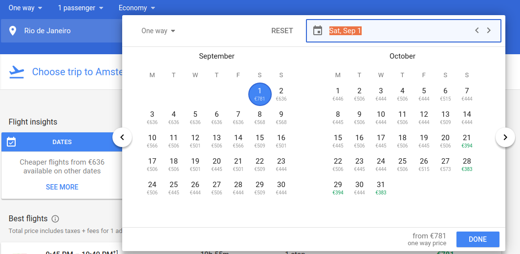
Apparently, there’s no open API for getting information about flights. But as Google Flights can show a calendar with prices for dates for two months I decided to use it:

Calendar with prices

So I’ve generated every possible combination of interesting destinations in South America and flights to and from Amsterdam. Simulated user interaction with changing destination inputs and opening/closing calendar. By the end, I wrote results as JSON in a new tab. The whole code isn’t that interesting and available in the gist. From the high level it looks like:

const getFlightsData = async ([from, to]) => {
  await setDestination(FROM, from);
  await setDestination(TO, to);

  const prices = await getPrices();

  return prices.map(([date, price]) => ({
    date, price, from, to,
  }));
};

const collectData = async () => {
  let result = [];
  for (let flight of getAllPossibleFlights()) {
    const flightsData = await getFlightsData(flight);
    result = result.concat(flightsData);
  }
  return result;
};

const win = window.open('');

collectData().then(
  (data) => win.document.write(JSON.stringify(data)),
  (error) => console.error("Can't get flights", error),
);

In action:

I’ve run it twice to have separate data for flights with and without stops, and just saved the result to JSON files with content like:

[{"date":"2018-07-05","price":476,"from":"Rio de Janeiro","to":"Montevideo"},
{"date":"2018-07-06","price":470,"from":"Rio de Janeiro","to":"Montevideo"},
{"date":"2018-07-07","price":476,"from":"Rio de Janeiro","to":"Montevideo"},
...]

Although, it mostly works, in some rare cases it looks like Google Flights has some sort of anti-parser and show “random” prices.

Selecting the best trips

In the previous part, I’ve parsed 10110 flights with stop and 6422 non-stop flights, it’s impossible to use brute force algorithm here (I’ve tried). As reading data from JSON isn’t interesting, I’ll skip that part.

At first, I’ve built an index of from destinationdayto destination:

from_id2day_number2to_id2flight = defaultdict(
    lambda: defaultdict(
        lambda: {}))
for flight in flights:
    from_id2day_number2to_id2flight[flight.from_id] \
        [flight.day_number][flight.to_id] = flight

Created a recursive generator that creates all possible trips:

def _generate_trips(can_visit, can_travel, can_spent, current_id,
                    current_day, trip_flights):
    # The last flight is to home city, the end of the trip
    if trip_flights[-1].to_id == home_city_id:
        yield Trip(
            price=sum(flight.price for flight in trip_flights),
            flights=trip_flights)
        return

    # Everything visited or no vacation days left or no money left
    if not can_visit or can_travel < MIN_STAY or can_spent == 0:
        return

    # The minimal amount of cities visited, can start "thinking" about going home
    if len(trip_flights) >= MIN_VISITED and home_city_id not in can_visit:
        can_visit.add(home_city_id)

    for to_id in can_visit:
        can_visit_next = can_visit.difference({to_id})
        for stay in range(MIN_STAY, min(MAX_STAY, can_travel) + 1):
            current_day_next = current_day + stay
            flight_next = from_id2day_number2to_id2flight \
                .get(current_id, {}).get(current_day_next, {}).get(to_id)
            if not flight_next:
                continue

            can_spent_next = can_spent - flight_next.price
            if can_spent_next < 0:
                continue

            yield from _generate_trips(
                can_visit_next, can_travel - stay, can_spent_next, to_id,
                                current_day + stay, trip_flights + [flight_next])

As the algorithm is easy to parallel, I’ve made it possible to run with Pool.pool.imap_unordered, and pre-sort for future sorting with merge sort:

def _generator_stage(params):
    return sorted(_generate_trips(*params), key=itemgetter(0))

Then generated initial flights and other trip flights in parallel:

def generate_trips():
    generators_params = [(
        city_ids.difference({start_id, home_city_id}),
        MAX_TRIP,
        MAX_TRIP_PRICE - from_id2day_number2to_id2flight[home_city_id][start_day][start_id].price,
        start_id,
        start_day,
        [from_id2day_number2to_id2flight[home_city_id][start_day][start_id]])
        for start_day in range((MAX_START - MIN_START).days)
        for start_id in from_id2day_number2to_id2flight[home_city_id][start_day].keys()]

    with Pool(cpu_count() * 2) as pool:
        for n, stage_result in enumerate(pool.imap_unordered(_generator_stage, generators_pa
rams)):
            yield stage_result

And sorted everything with heapq.merge:

trips = [*merge(*generate_trips(), key=itemgetter(0))]

Looks like a solution to a job interview question.

Without optimizations, it was taking more than an hour and consumed almost whole RAM (apparently typing.NamedTuple isn’t memory efficient with multiprocessing at all), but current implementation takes 1 minute 22 seconds on my laptop.

As the last step I’ve saved results in csv (the code isn’t interesting and available in the gist), like:

price,days,cities,start city,start date,end city,end date,details
1373,15,4,La Paz,2018-09-15,Buenos Aires,2018-09-30,Amsterdam -> La Paz 2018-09-15 498 & La Paz -> Santiago 2018-09-18 196 & Santiago -> Montevideo 2018-09-23 99 & Montevideo -> Buenos Aires 2018-09-26 120 & Buenos Aires -> Amsterdam 2018-09-30 460
1373,15,4,La Paz,2018-09-15,Buenos Aires,2018-09-30,Amsterdam -> La Paz 2018-09-15 498 & La Paz -> Santiago 2018-09-18 196 & Santiago -> Montevideo 2018-09-23 99 & Montevideo -> Buenos Aires 2018-09-27 120 & Buenos Aires -> Amsterdam 2018-09-30 460
1373,15,4,La Paz,2018-09-15,Buenos Aires,2018-09-30,Amsterdam -> La Paz 2018-09-15 498 & La Paz -> Santiago 2018-09-20 196 & Santiago -> Montevideo 2018-09-23 99 & Montevideo -> Buenos Aires 2018-09-26 120 & Buenos Aires -> Amsterdam 2018-09-30 460
1373,15,4,La Paz,2018-09-15,Buenos Aires,2018-09-30,Amsterdam -> La Paz 2018-09-15 498 & La Paz -> Santiago 2018-09-20 196 & Santiago -> Montevideo 2018-09-23 99 & Montevideo -> Buenos Aires 2018-09-27 120 & Buenos Aires -> Amsterdam 2018-09-30 460
...

Gist with sources.

Filmstrip from subtitles and stock images


It’s possible to find subtitles for almost every movie or TV series. And there’s also stock images with anything imaginable. Wouldn’t it be fun to connect this two things and make a sort of a filmstrip with a stock image for every caption from subtitles?

TLDR: the result is silly:

For the subtitles to play with I chose subtitles for Bob’s Burgers – The Deeping. At first, we need to parse it with pycaption:

from pycaption.srt import SRTReader

lang = 'en-US'
path = 'burgers.srt'

def read_subtitles(path, lang):
    with open(path) as f:
        data = f.read()
        return SRTReader().read(data, lang=lang)
        
        
subtitles = read_subtitles(path, lang)
captions = subtitles.get_captions(lang)
>>> captions
['00:00:04.745 --> 00:00:06.746\nShh.', '00:00:10.166 --> 00:00:20.484\n...

As a lot of subtitles contains html, it’s important to remove tags before future processing, it’s very easy to do with lxml:

import lxml.html

def to_text(raw_text):
    return lxml.html.document_fromstring(raw_text).text_content()
to_text('<i>That shark is ruining</i>')
'That shark is ruining'

For finding most significant words in the text we need to tokenize it, lemmatize (replace every different form of a word with a common form) and remove stop words. It’s easy to do with NLTK:

from nltk.corpus import stopwords
from nltk.tokenize import word_tokenize
from nltk.stem import WordNetLemmatizer

def tokenize_lemmatize(text):
    tokens = word_tokenize(text)
    lemmatizer = WordNetLemmatizer()
    lemmatized = [lemmatizer.lemmatize(token.lower())
                  for token in tokens if token.isalpha()]
    stop_words = set(stopwords.words("english"))
    return [lemma for lemma in lemmatized if lemma not in stop_words]
>>> tokenize_lemmatize('That shark is ruining')
['shark', 'ruining']

And after that we can just combine the previous two functions and find most frequently used words:

from collections import Counter

def get_most_popular(captions):
    full_text = '\n'.join(to_text(caption.get_text()) for caption in captions)
    tokens = tokenize_lemmatize(full_text)
    return Counter(tokens)
    
  
most_popular = get_most_popular(captions)
most_popular
Counter({'shark': 68, 'oh': 32, 'bob': 29, 'yeah': 25, 'right': 20,...

It’s not the best way to find the most important words, but it kind of works.

After that it’s straightforward to extract keywords from a single caption:

def get_keywords(most_popular, text, n=2):
    tokens = sorted(tokenize_lemmatize(text), key=lambda x: -most_popular[x])
    return tokens[:n]
>>> captions[127].get_text()
'Teddy, what is wrong with you?'
>>> get_keywords(most_popular, to_text(captions[127].get_text()))
['teddy', 'wrong']

The next step is to find a stock image for those keywords. There’s not that many properly working and documented stocks, so I chose to use Shutterstock API. It’s limited to 250 requests per hour, but it’s enough to play.

From their API we only need to use /images/search. We will search for the most popular photo:

import requests

# Key and secret of your app
stock_key = ''
stock_secret = ''

def get_stock_image_url(query):
    response = requests.get(
        "https://api.shutterstock.com/v2/images/search",
        params={
            'query': query,
            'sort': 'popular',
            'view': 'minimal',
            'safe': 'false',
            'per_page': '1',
            'image_type': 'photo',
        },
        auth=(stock_key, stock_secret),
    )
    data = response.json()
    try:
        return data['data'][0]['assets']['preview']['url']
    except (IndexError, KeyError):
        return None
>>> get_stock_image_url('teddy wrong')
'https://image.shutterstock.com/display_pic_with_logo/2780032/635833889/stock-photo-guilty-boyfriend-asking-for-forgiveness-presenting-offended-girlfriend-a-teddy-bear-toy-lady-635833889.jpg'

The image looks relevant:

teddy wrong

Now we can create a proper card from a caption:

def make_slide(most_popular, caption):
    text = to_text(caption.get_text())
    if not text:
        return None

    keywords = get_keywords(most_popular, text)
    query = ' '.join(keywords)
    if not query:
        return None

    stock_image = get_stock_image_url(query)
    if not stock_image:
        return None

    return text, stock_image
make_slide(most_popular, captions[132])
('He really chewed it...\nwith his shark teeth.', 'https://image.shutterstock.com/display_pic_with_logo/181702384/710357305/stock-photo-scuba-diver-has-shark-swim-really-close-just-above-head-as-she-faces-camera-below-710357305.jpg')

The image is kind of relevant:

He really chewed it...with his shark teeth.

After that we can select captions that we want to put in our filmstrip and generate html like the one in the TLDR section:

output_path = 'burgers.html'
start_slide = 98
end_slide = 200


def make_html_output(slides):
    html = '<html><head><link rel="stylesheet" href="./style.css"></head><body>'
    for (text, stock_image) in slides:
        html += f'''<div class="box">
            <img src="{stock_image}" />
            <span>{text}</span>
        </div>'''
    html += '</body></html>'
    return html


interesting_slides = [make_slide(most_popular, caption)
                      for caption in captions[start_slide:end_slide]]
interesting_slides = [slide for slide in interesting_slides if slide]

with open(output_path, 'w') as f:
    output = make_html_output(interesting_slides)
    f.write(output)

And the result - burgers.html.

Another example, even worse and a bit NSFW, It’s Always Sunny in Philadelphia – Charlie Catches a Leprechaun.

Gist with the sources.

Analyzing commute with Google Location History and Python


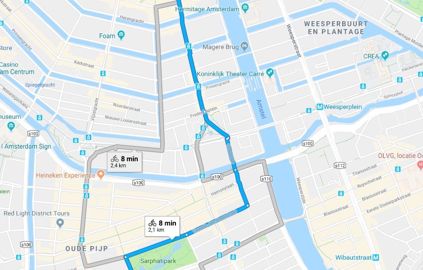
Map with commute

The article was updated 17.05.2018 with wind direction data.

Since I moved to Amsterdam I’m biking to work almost every morning. And as Google is always tracking the location of my phone, I thought that it might be interesting to do something with that data.

First of all, I’ve downloaded Location History data dump in json from Download your data page. The format of the dump is very simple, it’s a dict with locations key that contains a lot of entries like this in descendant order by date:

{
    "timestampMs" : "1525120611682",
    "latitudeE7" : 523508799,
    "longitudeE7" : 488938179,
    "accuracy" : 15,
    "altitude" : 49,
    "verticalAccuracy" : 2
}

It’s very easy to parse it with Python:

import json
from datetime import datetime
from collections import namedtuple

Point = namedtuple('Point', 'latitude, longitude, datetime')


def read_points():
    with open('data.json') as f:
        data = json.load(f)

    for point in data['locations']:
        yield Point(
            point['latitudeE7'] / 10 ** 7,
            point['longitudeE7'] / 10 ** 7,
            datetime.fromtimestamp(int(point['timestampMs']) / 1000)
        )
        
points = read_points()
>>> [*points]
[Point(latitude=52.350879, longitude=4.893817, datetime=datetime.datetime(2018, 4, 30, 22, 36, 51, 682000)), ...]

As I moved to my current place in November, it’s safe to ignore all entries before:

from itertools import takewhile

from_date = datetime(2017, 11, 1)

after_move = takewhile(lambda point: point.datetime >= from_date, points)

And weekends:

work_days = (point for point in after_move
             if point.datetime.weekday() < 5)

Usually, I’m heading to work between 9 am and 10 am, but as the Netherlands are switching between summer and winter timezones, it will be safer to treat everything between 7 am and 9a m as possible commute time:

from_hour = 7
to_hour = 12

commute_time = (point for point in work_days
                if from_hour <= point.datetime.hour < to_hour)

Then I grouped everything by date:

from itertools import groupby

by_days = groupby(commute_time, key=lambda point: point.datetime.date())
>>> [(day, [*vals]) for day, vals in by_days]
[(datetime.date(2018, 4, 27),
 [Point(latitude=52.350879, longitude=4.893817, datetime=datetime.datetime(2018, 4, 27, 11, 58, 17, 189000)), ...]),
 ...]

After that, I selected the last point at home and the first point at work for every day. A point considered home or work if it’s distance from home or work is smaller than 50 meters. The distance can be easily calculated with geopy:

from geopy.distance import geodesic

home = (52.350879, 4.893817)  # not really =)
work = (52.3657573, 4.8980648)

max_distance = 0.050

def last_at_home(points):
    result = None
    for point in points:
        if geodesic(home, point[:2]).km <= max_distance:
            result = point
    return result


def first_at_work(points, after):
    for point in points:
        if point.datetime > after.datetime and geodesic(work, point[:2]).km <= max_distance:
            return point


Commute = namedtuple('Commute', 'day, start, end, took')


def get_commute():
    for day, points in by_days:
        points = [*points][::-1]

        start = last_at_home(points)
        if start is None:
            continue

        end = first_at_work(points, start)
        if end is None:
            continue

        yield Commute(
            day, start.datetime, end.datetime, end.datetime - start.datetime,
        )


commutes = [*get_commute()][::-1]
>>> commutes
[Commute(day=datetime.date(2017, 11, 2), start=datetime.datetime(2017, 11, 2, 9, 39, 13, 219000), end=datetime.datetime(2017, 11, 2, 9, 52, 53, 295000), took=datetime.timedelta(0, 820, 76000)), ...]

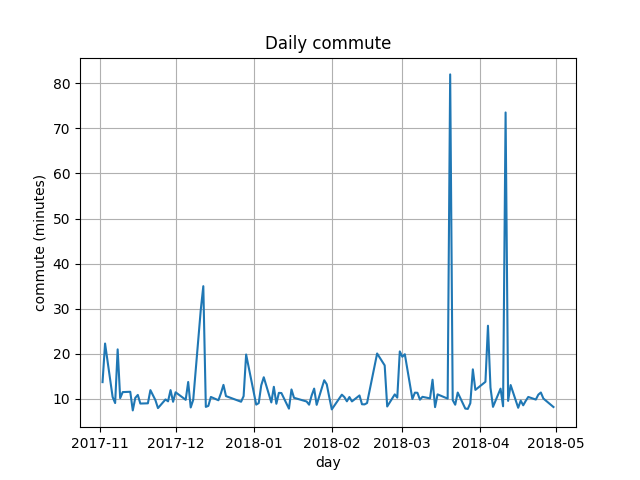
Now it’s easy to plot a graph of daily commute with matplotlib:

from matplotlib import pyplot

fig, ax = pyplot.subplots()
ax.plot([commute.day for commute in commutes],
        [commute.took.total_seconds() / 60 for commute in commutes])

ax.set(xlabel='day', ylabel='commute (minutes)',
       title='Daily commute')
ax.grid()
pyplot.show()

It’s easy to spot days when I had appointments in the morning:

Daily commute

Then I thought that it might be interesting to look for a correlation between temperature and commute time, and wind speed and commute time. I found data dump of daily weather that KNMI provides, the nearest meteorological station is in Schiphol airport, but I guess it’s close enough. The data is in easy to parse format:

# STN,YYYYMMDD,DDVEC,FHVEC,   FG,  FHX, FHXH,  FHN, FHNH,  FXX, FXXH,   TG,   TN,  TNH,   TX,  TXH, T10N,T10NH,   SQ,   SP,    Q,   DR,   RH,  RHX, RHXH,   PG,   PX,  PXH,   PN,  PNH,  VVN, VVNH,  VVX, VVXH,   NG,   UG,   UX,  UXH,   UN,  UNH, EV24

  240,19510101,  188,   77,   87,  195,   18,   41,   24,     ,     ,   12,  -13,    1,   26,   20,     ,     ,     ,     ,     ,     ,     ,     ,     , 9891, 9957,     , 9837,     ,     ,     ,     ,     ,    7,   90,   98,    6,   73,   20,     
  240,19510102,  153,   41,   41,   82,    4,   10,   21,     ,     ,   13,    7,    4,   18,   19,     ,     ,     ,     ,     ,     ,     ,     ,     , 9876, 9923,     , 9853,     ,     ,     ,     ,     ,    8,   93,   98,    9,   88,    1,     

I only used FG (Daily mean wind speed in 0.1 m/s), TG (Daily mean temperature in 0.1 degrees Celsius) and DDVEC (Vector mean wind direction in degrees):

from dateutil.parser import parse

Weather = namedtuple('Weather', 'windspeed, temperature, wind_direction')


def read_weather():
    result = {}

    with open('weather.txt') as f:
        for line in f.readlines():
            if not line.startswith(' '):
                continue

            data = [part.strip() for part in line.split(',')]
            result[parse(data[1]).date()] = Weather(
                int(data[4]) / 10,
                int(data[11]) / 10,
                int(data[2]),
            )

    return result

weather = read_weather()
>>> weather
{datetime.date(1951, 1, 1): Weather(windspeed=8.7, temperature=1.2, wind_direction=188),
 datetime.date(1951, 1, 2): Weather(windspeed=4.1, temperature=1.3, wind_direction=153),
 datetime.date(1951, 1, 3): Weather(windspeed=2.1, temperature=0.3, wind_direction=203),
 ...}

Before doing this I’ve excluded spikes from days when I had appointments:

normalized = [commute for commute in commutes
              if commute.took.total_seconds() < 60 * 20]

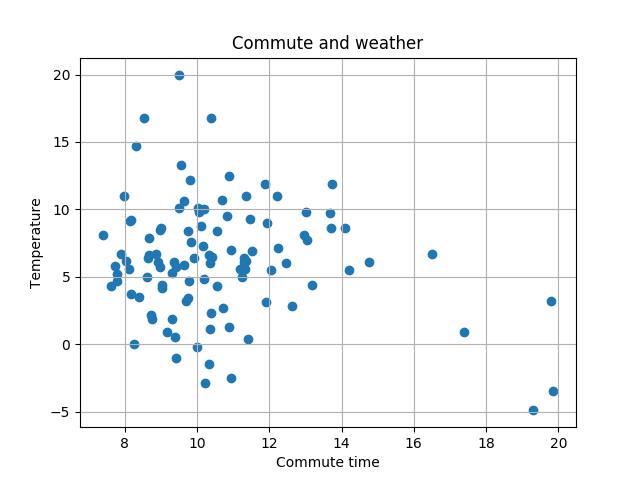
Then I created a scatter plot of temperature and commute:

fig, ax = pyplot.subplots()
ax.grid()
ax.scatter([commute.took.total_seconds() / 60 for commute in normalized],
           [weather[commute.day].temperature for commute in normalized])
ax.set(xlabel='Commute time', ylabel='Temperature',
       title='Commute and weather')
ax.legend()
pyplot.show()

Correlation is slightly visible, on cold days commute is a bit faster:

Commute and temperature

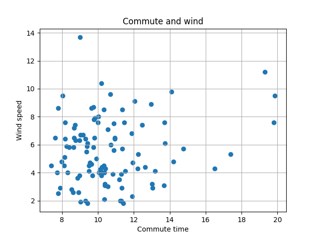
With wind speed code is almost the same:

fig, ax = pyplot.subplots()
ax.grid()
ax.scatter([commute.took.total_seconds() / 60 for commute in normalized],
           [weather[commute.day].windspeed for commute in normalized])
ax.set(xlabel='Commute time', ylabel='Wind speed',
       title='Commute and wind')
ax.legend()
pyplot.show()

And the correlation is more visible, the commute is slower with stronger wind:

Commute and wind

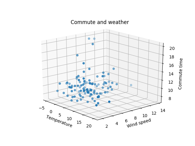
Then I’ve tried to combine the previous two graphs in one 3d graph:

from mpl_toolkits.mplot3d import Axes3D

fig, ax = pyplot.subplots(subplot_kw={'projection': '3d'})
ax.grid()
ax.scatter([weather[commute.day].temperature for commute in normalized],
           [weather[commute.day].windspeed for commute in normalized],
           [commute.took.total_seconds() / 60 for commute in normalized])
ax.set(xlabel='Temperature', ylabel='Wind speed', zlabel='Commute time',
       title='Commute and weather')
ax.legend()
pyplot.show()

And the result didn’t give me anything:

Commute and weather in 3d

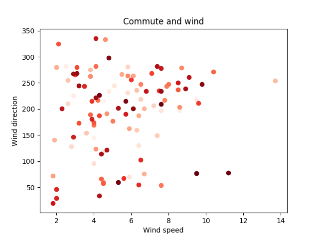
After that I thought that it would be interesting to look at a possible correlation of commute time, wind speed, and direction:

from matplotlib import cm

colors = iter(cm.Reds(np.linspace(0, 1, len(normalized))))

fig, ax = pyplot.subplots()
ax.grid()

for commute in sorted(normalized, key=lambda commute: commute.took.total_seconds() / 60):
    ax.scatter(weather[commute.day].windspeed,
               weather[commute.day].wind_direction,
               color=next(colors))

ax.set(xlabel='Wind speed', ylabel='Wind direction',
       title='Commute and wind')

ax.grid()

pyplot.show()

Longer the commute, redder the dot:

Commute, wind speed and direction

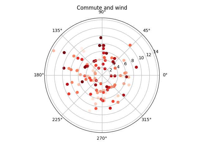
Wind direction doesn’t look that well on that plot, so I’ve tried to use polar plot:

colors = iter(cm.Reds(np.linspace(0, 1, len(normalized))))

fig, ax = pyplot.subplots(subplot_kw={'projection': 'polar'})

for commute in sorted(normalized, key=lambda commute: commute.took.total_seconds() / 60):
    ax.scatter(weather[commute.day].wind_direction,
               weather[commute.day].windspeed,
               color=next(colors))

ax.set(title='Commute and wind')

ax.grid()

pyplot.show()

And it’s much more “readable”:

Polar commute, wind speed and direction

Gist with sources.

Alan A. A. Donovan,‎ Brian W. Kernighan: The Go Programming Language


book cover white Somehow I’ve started to use Go more and more, so I decided to read something fundamental about it. The Go Programming Language by Alan A. A. Donovan and‎ Brian W. Kernighan looked like a right choice. The book covers every aspect of the language from very basic things like statements and variables to reflection and interop with C. It also covers some best practices, and things that better not to do.

Although I’m not a big fan of Go and it’s best practices, the book at least helped me to understand why it’s done that way a bit better.

Rob Fitzpatrick: The Mom Test


book cover Recently I wanted to read something that can help with meetings and talks with non-technical people. And I was recommended to read The Mom Test by Rob Fitzpatrick. It’s a short book and it’s an easy reading, the book has a few valid points and ideas. It explains author’s points by showing example dialogs with highlighted bad and good parts.

From the other side, the book gives too startup-ish/entrepreneur-ish in a bad way aftertaste.

Anil Madhavapeddy, Jason Hickey, Yaron Minsky: Real World OCaml


book cover white Around a month ago I’ve started playing around Reason and for understanding it better I decided to read something about OCaml and chose Real World OCaml by Anil Madhavapeddy, Jason Hickey, and Yaron Minsky. The book explains OCaml syntax, core library, different aspects of language and how to write FP and OOP code in OCaml. The book has a lot of examples and easy to read, not that much repetitive as a lot of books about programming languages.

Although before reading the book I thought that OCaml isn’t that much over-bloated and is a better language, especially it’s syntax. It helped me to better understand concepts and ideas behind Reason.

Don Norman: The Design of Everyday Things


book cover Recently I wanted to read something about UI and UX and I was recommended to read The Design of Everyday Things by Don Norman. Even I’m not a UI/UX specialist at all, it’s one of the most interesting books I’ve read lately. It contains a lot of real-life examples with deep explanations why something is done wrongly and poorly, and it has points and ideas how to make it better.

Although the book is a bit repetitive.

James Turnbull: The Logstash Book


book cover white As I have an interest in monitoring and logging, I decided to read The Logstash Book by James Turnbull. And it’s kind of a nice book, with examples and explanations about working with Logstash and ELK stack. Also, it contains information about the ways to extend Logstash with plugins, even a few pages about writing plugins on your own.

From the other side, the book is a bit too basic and a lot of it is primitive information about deploying Logstash and related stack.